  ID time age drug status    entdate    enddate
1  1    5  46    0      1 15/05/2015 14/10/2015
2  2    6  35    1      0 19/09/2014 20/03/2015
3  3    8  30    1      1 21/04/2016 20/12/2016
4  4    3  30    1      1 03/01/2016 04/04/2016
5  5   22  36    0      1 18/09/2014 19/07/2016
6 6 1 32 1 0 18/03/2016 17/04/2016Lab 7: Kaplan–Meier estimate of the survival functions and Cox regression model
\[ \renewcommand{\P}{\mathbb{P}} \newcommand{\E}{\mathbb{E}} \]
1 Reminder about data frames
1.1
Download hm.csv, store it in a variable df, and display the first rows of the dataset.
This data frame contains information about patients participating in a clinical trial.
time: duration of follow-up (in months)age: age of the participantdrug: treatment indicator (0= no drug,1= drug)status: event indicator:1= event of interest observed0= censored observation
In this dataset, the event of interest is death related to the condition under study.
If a patient dies from an unrelated cause, or leaves the study early, the observation is censored: we only know that the patient survived at least up to that time.
1.2
Find the mean age of the participants.
[1] 36.071.3
Find the number of observations (rows) in the dataset.
[1] 1002 Kaplan–Meier estimate
We use the package survival (you may need to install it, see Lab 2 on how to install a package).
library(survival)To work with survival data, we first create a survival object using Surv():
sf <- Surv(df$time, df$status)
sf
[1] 5 6+ 8 3 22 1+ 7 9 3 12 2+ 12 1 15 34 1 4 19+
[19] 3+ 2 2+ 6 60+ 11 2+ 5 4+ 1 13 3 2 1 30 7 4 8
[37] 5 10 2 9 36 3 9 3 35 8 11 56+ 2+ 3 15 1 10 1
[55] 7 3 3 2 32 3 10+ 11 3 7 5 31 5 58 1 3+ 43 1
[73] 6 53 14 4 54 1 1 8 5 1 1 2 7+ 1+ 10 24+ 7 12+
[91] 4 57 1 12+ 7 1 5 60+ 2+ 1 Censored observations are marked with a +. This means that the event was not observed at that time.
We now compute the Kaplan–Meier estimator:
km <- survfit(sf ~ 1)
km
Call: survfit(formula = sf ~ 1)
n events median 0.95LCL 0.95UCL
[1,] 100 80 7 5 10The formula ~ 1 means that we estimate a single survival curve for the whole sample, without using any covariates.
Plotting the estimator:
plot(km)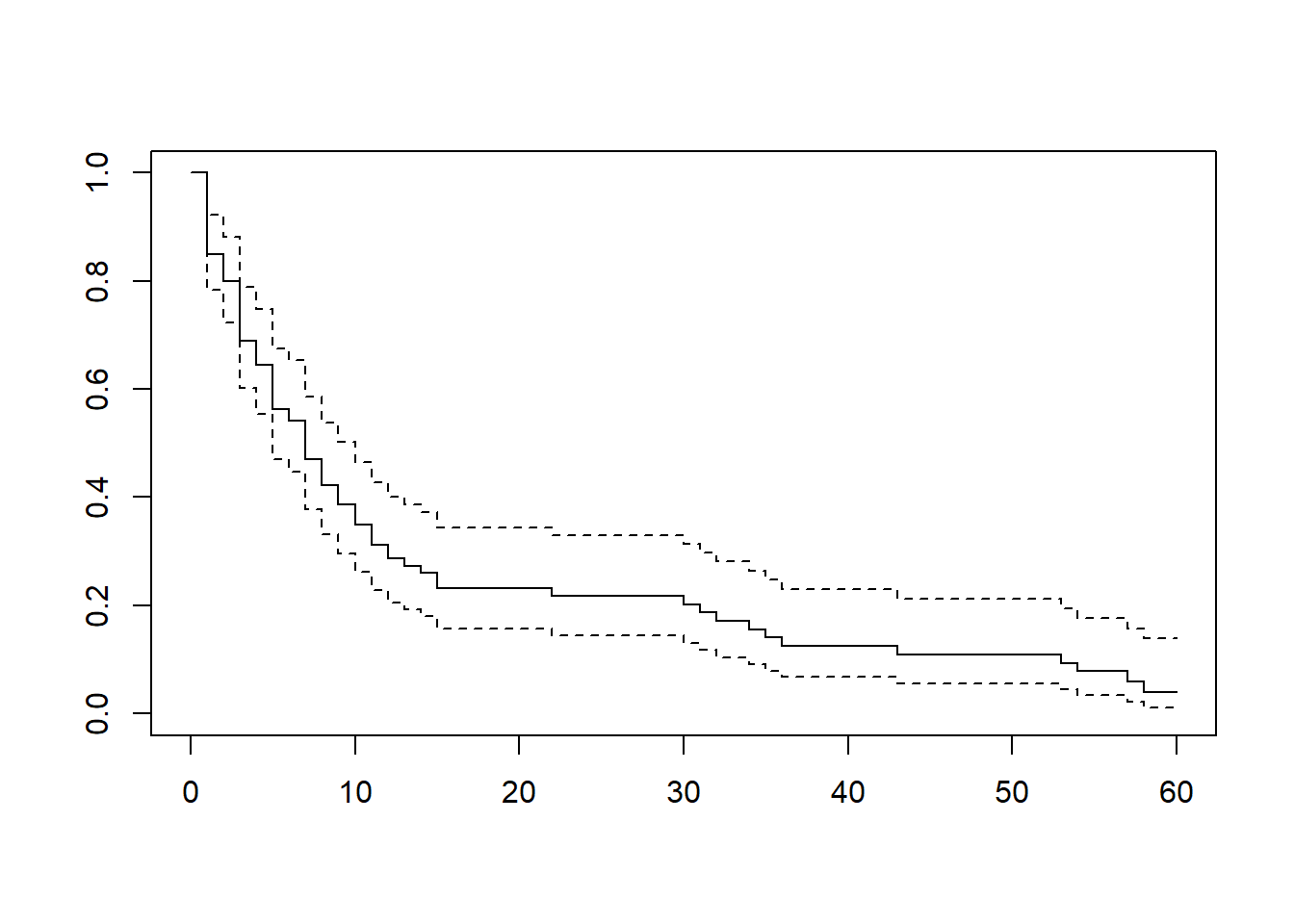
The solid line is the Kaplan–Meier estimate \(\hat{S}(t)\)
The dashed lines represent a \(95\)% confidence interval
Roughly speaking, if we repeated the study many times, the true survival probabilities would lie within these bounds in about \(95\)% of cases.
To change the confidence level, we the paramter
conf.int=valueof functionplotwherevalueis a decimal between \(0\) and \(1\).Higher confidence level → wider interval.
Numerical values:
summary(km)Call: survfit(formula = sf ~ 1)
time n.risk n.event survival std.err lower 95% CI upper 95% CI
1 100 15 0.8500 0.0357 0.7828 0.923
2 83 5 0.7988 0.0402 0.7237 0.882
3 73 10 0.6894 0.0473 0.6026 0.789
4 61 4 0.6442 0.0493 0.5544 0.748
5 56 7 0.5636 0.0517 0.4709 0.675
6 49 2 0.5406 0.0521 0.4476 0.653
7 46 6 0.4701 0.0526 0.3775 0.586
8 39 4 0.4219 0.0525 0.3306 0.538
9 35 3 0.3857 0.0520 0.2962 0.502
10 32 3 0.3496 0.0511 0.2625 0.466
11 28 3 0.3121 0.0500 0.2280 0.427
12 25 2 0.2872 0.0490 0.2055 0.401
13 21 1 0.2735 0.0486 0.1931 0.387
14 20 1 0.2598 0.0480 0.1809 0.373
15 19 2 0.2325 0.0467 0.1568 0.345
22 16 1 0.2179 0.0460 0.1441 0.330
30 14 1 0.2024 0.0453 0.1305 0.314
31 13 1 0.1868 0.0444 0.1173 0.298
32 12 1 0.1712 0.0433 0.1043 0.281
34 11 1 0.1557 0.0421 0.0916 0.264
35 10 1 0.1401 0.0407 0.0793 0.247
36 9 1 0.1245 0.0390 0.0674 0.230
43 8 1 0.1090 0.0371 0.0559 0.212
53 7 1 0.0934 0.0349 0.0449 0.194
54 6 1 0.0778 0.0324 0.0344 0.176
57 4 1 0.0584 0.0296 0.0216 0.157
58 3 1 0.0389 0.0253 0.0109 0.139* `time`: event times
* `n.risk`: individuals at risk just before time
* `n.event`: number of events at that time
* `surv`: estimated survival probabilityRecall that the Kaplan–Meier estimator is
\[ \hat{S}(t) = \prod_{t_j \le t} \left(1 - \frac{d_j}{n_j}\right). \]
Extracting survival probabilities
Instead of reading values manually, we can query the model:
summary(km, times = c(13, 42))$surv[1] 0.2734790 0.12453062.1
Compute the ratio \[ \frac{\hat{S}(17)}{\hat{S}(51)}. \]
[1] 2.1333332.2
Find the estimated probability of the death in the next \(2\) years.
[1] 0.7820714Median survival time
kmCall: survfit(formula = sf ~ 1)
n events median 0.95LCL 0.95UCL
[1,] 100 80 7 5 10The output includes the median survival time, i.e. the time when \(\hat{S}(t) = 0.5\).
3 Kaplan–Meier with covariates
We now compare groups:
kmdrug <- survfit(sf ~ df$drug)
kmdrug
Call: survfit(formula = sf ~ df$drug)
n events median 0.95LCL 0.95UCL
df$drug=0 51 42 11 8 30
df$drug=1 49 38 5 3 7plot(kmdrug, col = c("blue", "red"))
legend("topright", legend = c("No drug", "Drug"),
col = c("blue", "red"), lty = c(1,1))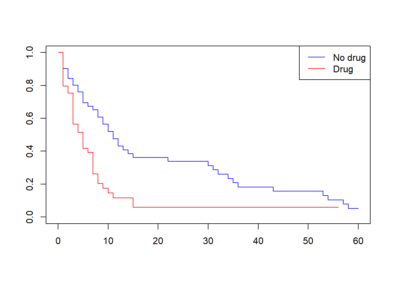
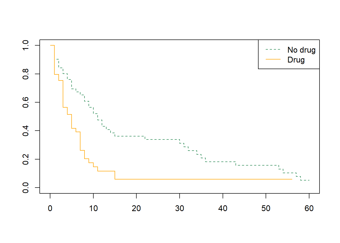
3.1
Modify the plot so that:
“No drug” is dashed seagreen
“Drug” is solid orange
Embedded data. The dataframe lung is embedded into survival package. You can get information about this data frame by typing in the console ?lung.
kmlung <- survfit(Surv(time, status == 2) ~ sex, data = lung)
kmlung
Call: survfit(formula = Surv(time, status == 2) ~ sex, data = lung)
n events median 0.95LCL 0.95UCL
sex=1 138 112 270 212 310
sex=2 90 53 426 348 550Here we explicitly define the event as status == 2 (death), which is clearer.
plot(kmlung, col = c("blue", "red"))
legend("topright", legend = c("Male", "Female"),
       col = c("blue", "red"), lty = c(1,1))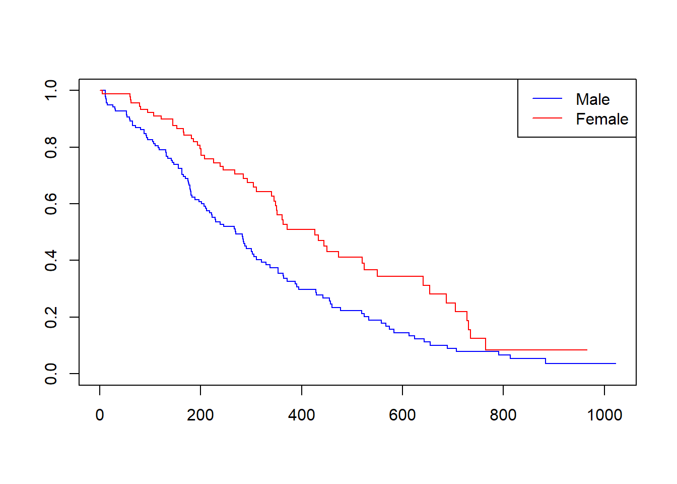
Surely, there are numerous R packages which can make plots more nice. For example, one can install and load survminer package:
library(survminer)
ggsurvplot(kmlung, conf.int = 0.95)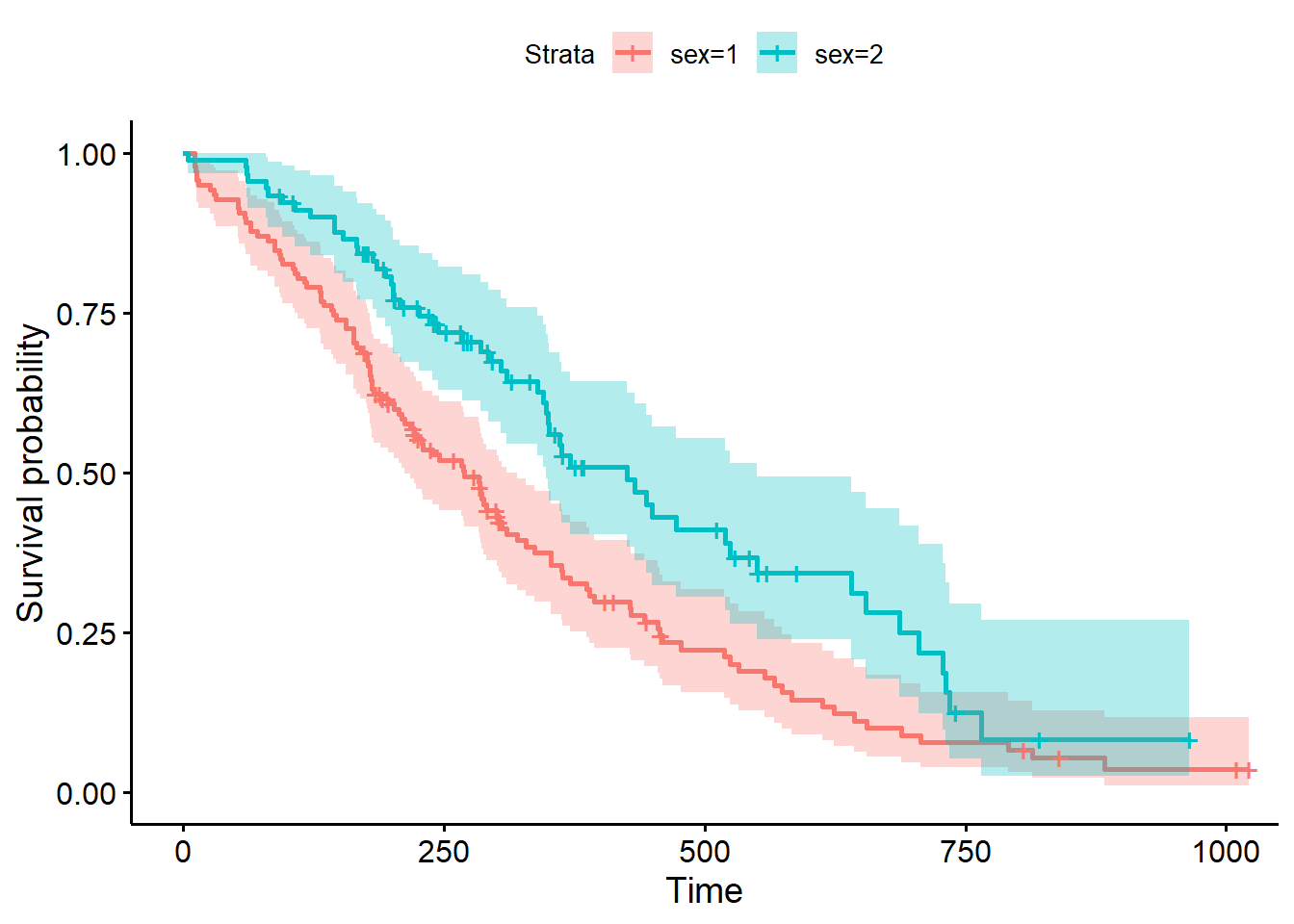
4 Cox regression model
The Cox model assumes:
\[ \lambda(t, z) = \lambda_0(t) e^{\beta z}. \]
It assumes proportional hazards, meaning hazard ratios do not depend on time.
One covariate case
fit <- coxph(Surv(time, status == 2) ~ sex, data = lung)
summary(fit)
Call:
coxph(formula = Surv(time, status == 2) ~ sex, data = lung)
n= 228, number of events= 165
coef exp(coef) se(coef) z Pr(>|z|)
sex -0.5310 0.5880 0.1672 -3.176 0.00149 **
---
Signif. codes: 0 '***' 0.001 '**' 0.01 '*' 0.05 '.' 0.1 ' ' 1
exp(coef) exp(-coef) lower .95 upper .95
sex 0.588 1.701 0.4237 0.816
Concordance= 0.579 (se = 0.021 )
Likelihood ratio test= 10.63 on 1 df, p=0.001
Wald test = 10.09 on 1 df, p=0.001
Score (logrank) test = 10.33 on 1 df, p=0.001coef: estimate of \(\beta\)exp(coef): hazard ratio
Interpretation:
If exp(coef) = 0.588, then females have about 0.588 times the hazard of males (i.e. about 41% lower hazard).
Multiple covariates case
fit2 <- coxph(Surv(time, status == 2) ~ sex + age, data = lung)
summary(fit2)
Call:
coxph(formula = Surv(time, status == 2) ~ sex + age, data = lung)
n= 228, number of events= 165
coef exp(coef) se(coef) z Pr(>|z|)
sex -0.513219 0.598566 0.167458 -3.065 0.00218 **
age 0.017045 1.017191 0.009223 1.848 0.06459 .
---
Signif. codes: 0 '***' 0.001 '**' 0.01 '*' 0.05 '.' 0.1 ' ' 1
exp(coef) exp(-coef) lower .95 upper .95
sex 0.5986 1.6707 0.4311 0.8311
age 1.0172 0.9831 0.9990 1.0357
Concordance= 0.603 (se = 0.025 )
Likelihood ratio test= 14.12 on 2 df, p=9e-04
Wald test = 13.47 on 2 df, p=0.001
Score (logrank) test = 13.72 on 2 df, p=0.001For age:
b <- coef(fit2)
exp(b["age"])
age
1.017191 This gives the multiplicative increase per year.
4.1
Compute the hazard ratio for:
a male aged 70
a female aged 80
     sex
1.408838
Likelihood ratio test
A natural question is: when we used both age and gender covariates, we get different answers comparing with using eitehr of covariates alone. Does adding new covariates improve the model? More formally, let \(L_p\) be the likelihood function with \(p\in\mathbb{N}\) covariates and let \(L_{p+q}\) be the likelihood function with \(p+q\in\mathbb{N}\) covariates. How to estimate if \(q\) additional covariates were significant to add?
For this, one can use the statistical test. The test statistic is
\[ \lambda:= 2(l_{p+q}-l_p)=2(\ln L_{p+q}-\ln L_{p})=2\ln\frac{L_{p+q}}{L_p}>0, \]
where all functions are calculated at the points of their maximums. Note \(L_{p+q}>L_p\) because \(L_{p+q}\) is calculated at maximum over all possible \(p+q\) values, while \(L_p\) may be understood as the maximum of the function of \(p+q\) variables over the first \(p\) variables with fixed last \(q\) variables equal to \(0\):
\[ \beta_1 \cdot z_1+ \ldots +\beta_p \cdot z_p + 0\cdot z_{p+1} + \ldots + 0\cdot z_{p+q} =\beta_1 \cdot z_1+ \ldots +\beta_p \cdot z_p. \]
The \(H_0\) hypotehsis is then that \(\beta_{p+1}+\ldots+\beta_{p+q}=0\). The test is \(\chi^2\) test with \(q\) degrees of freedom:
fit1 <- coxph(Surv(time, status == 2) ~ sex, data = lung)
fit2 <- coxph(Surv(time, status == 2) ~ sex + age, data = lung)

anova(fit1, fit2, test = "LRT")
Analysis of Deviance Table
Cox model: response is Surv(time, status == 2)
Model 1: ~ sex
Model 2: ~ sex + age
loglik Chisq Df Pr(>|Chi|)
1 -744.59
2 -742.85 3.4895 1 0.06176 .
---
Signif. codes: 0 '***' 0.001 '**' 0.01 '*' 0.05 '.' 0.1 ' ' 1The number \(0.06176\) is the \(p\)-value. Hence, if we need the (standard) \(5\)% significance level, we do not regect the null hypothesis (as \(0.06176>0.05\)), so there is some evidence that age affects the hazard (after accounting for sex factor), but it is not strong enough at the \(5\)% level.
4.2
Check if sex affects the hazard here, at the \(5\)% level.
Check you answer: the \(p\)-value is \(0.001669<0.05\), hence, we reject the null hypothesis that sex does not affect the hazard, i.e. after accounting for age, sex does significantly improve the model.