This data frame contains information about patients participating in a clinical trial.
time: duration of follow-up (in months)
age: age of the participant
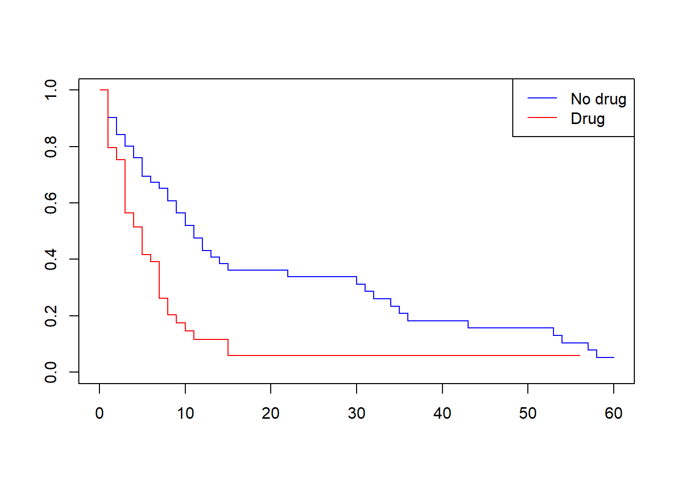
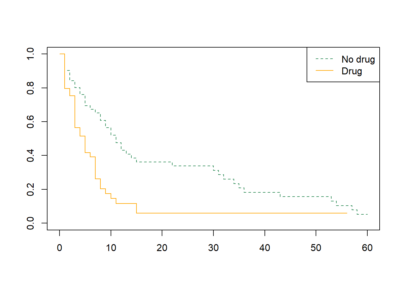
drug: treatment indicator (0 = no drug, 1 = drug)
status: event indicator:
1 = event of interest observed
0 = censored observation
In this dataset, the event of interest is death related to the condition under study.
If a patient dies from an unrelated cause, or leaves the study early, the observation is censored: we only know that the patient survived at least up to that time.
1.2
Find the mean age of the participants.
Code
mean(df$age)
[1] 36.07
1.3
Find the number of observations (rows) in the dataset.
Code
length(df$age)
[1] 100
Code
#or, better,
# nrow(df)
2 Kaplan–Meier estimate
We use the package survival (you may need to install it, see Lab 2 on how to install a package).
library(survival)
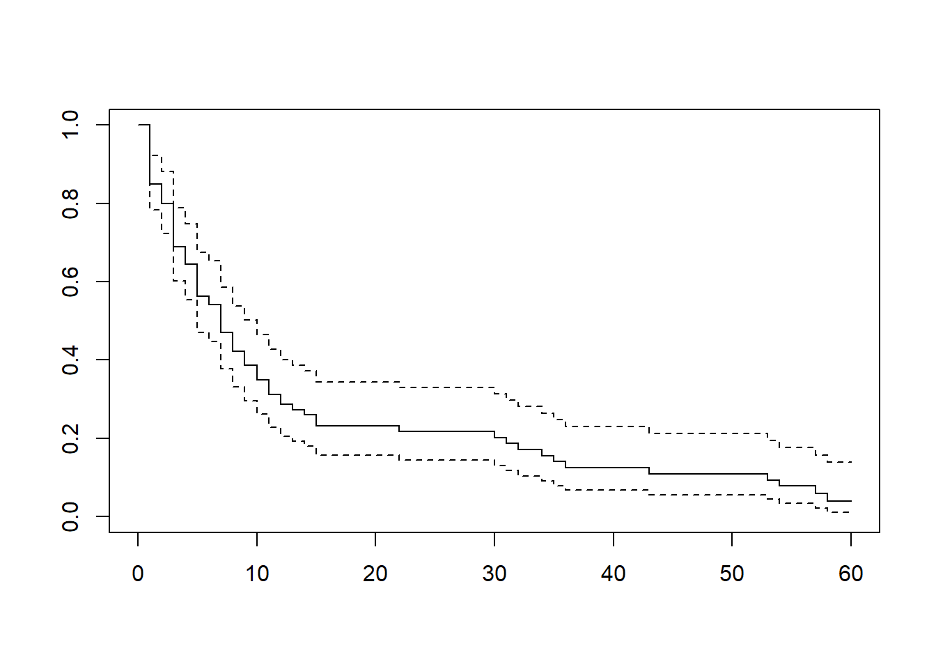
To work with survival data, we first create a survival object using Surv():
* `time`: event times

* `n.risk`: individuals at risk just before time

* `n.event`: number of events at that time

* `surv`: estimated survival probability
It assumes proportional hazards, meaning hazard ratios do not depend on time.
One covariate case
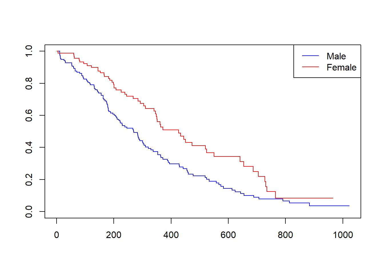
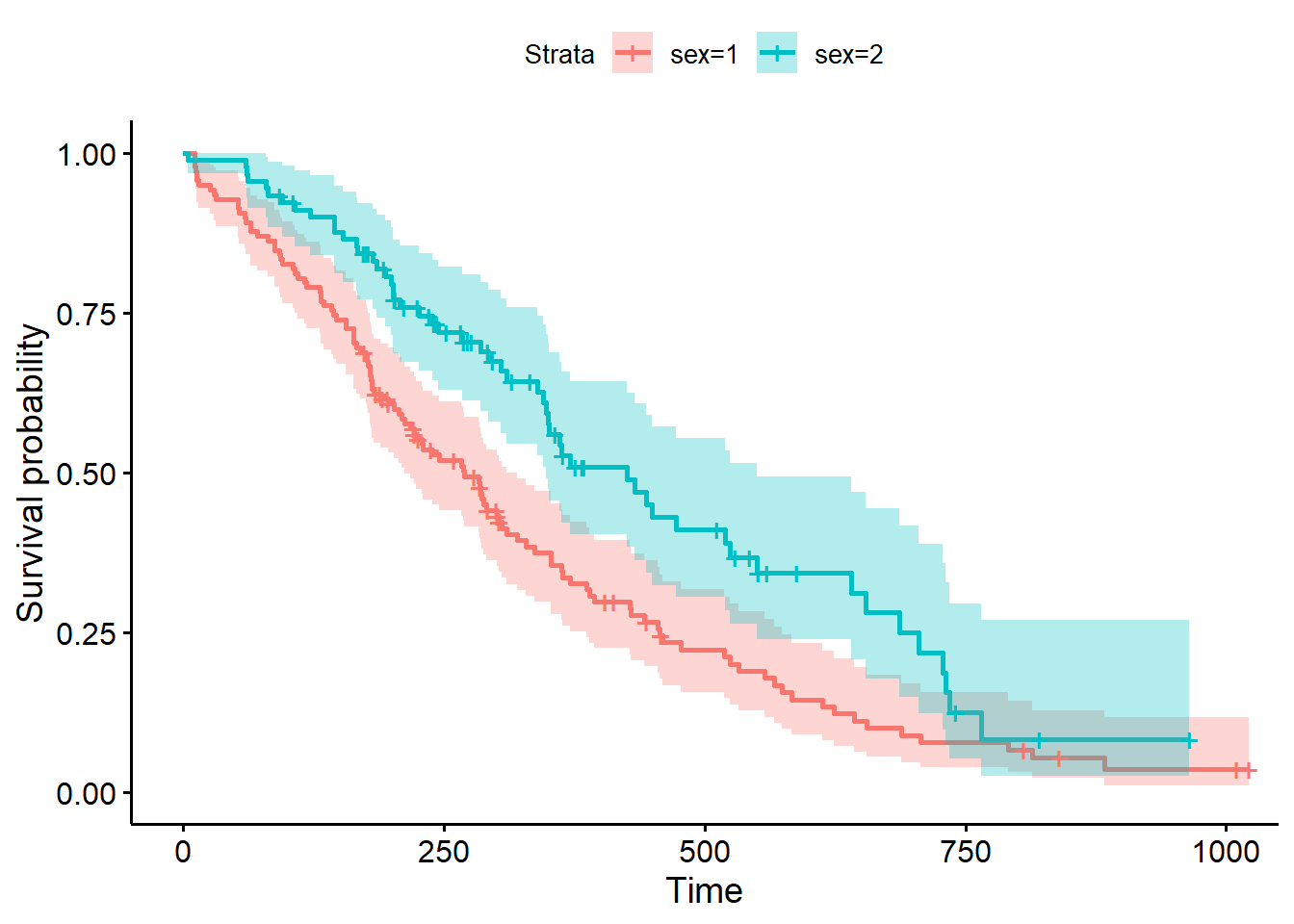
fit <-coxph(Surv(time, status ==2) ~ sex, data = lung)summary(fit)
Call:
coxph(formula = Surv(time, status == 2) ~ sex, data = lung)

  n= 228, number of events= 165

       coef exp(coef) se(coef)      z Pr(>|z|)
sex -0.5310    0.5880   0.1672 -3.176  0.00149 **
---
Signif. codes:  0 '***' 0.001 '**' 0.01 '*' 0.05 '.' 0.1 ' ' 1

    exp(coef) exp(-coef) lower .95 upper .95
sex     0.588      1.701    0.4237     0.816

Concordance= 0.579  (se = 0.021 )
Likelihood ratio test= 10.63  on 1 df,   p=0.001
Wald test            = 10.09  on 1 df,   p=0.001
Score (logrank) test = 10.33  on 1 df,   p=0.001
coef: estimate of \(\beta\)
exp(coef): hazard ratio
Interpretation:
If exp(coef) = 0.588, then females have about 0.588 times the hazard of males (i.e. about 41% lower hazard).
Multiple covariates case
fit2 <-coxph(Surv(time, status ==2) ~ sex + age, data = lung)summary(fit2)
Call:
coxph(formula = Surv(time, status == 2) ~ sex + age, data = lung)

  n= 228, number of events= 165

         coef exp(coef)  se(coef)      z Pr(>|z|)
sex -0.513219  0.598566  0.167458 -3.065  0.00218 **
age  0.017045  1.017191  0.009223  1.848  0.06459 .
---
Signif. codes:  0 '***' 0.001 '**' 0.01 '*' 0.05 '.' 0.1 ' ' 1

    exp(coef) exp(-coef) lower .95 upper .95
sex    0.5986     1.6707    0.4311    0.8311
age    1.0172     0.9831    0.9990    1.0357

Concordance= 0.603  (se = 0.025 )
Likelihood ratio test= 14.12  on 2 df,   p=9e-04
Wald test            = 13.47  on 2 df,   p=0.001
Score (logrank) test = 13.72  on 2 df,   p=0.001
For age:
b <-coef(fit2)exp(b["age"])
     age
1.017191
This gives the multiplicative increase per year.
4.1
Compute the hazard ratio for:
a male aged 70
a female aged 80
Code
exp(b["sex"]*(1-2) + b["age"]*(70-80))
     sex
1.408838
Likelihood ratio test
A natural question is: when we used both age and gender covariates, we get different answers comparing with using eitehr of covariates alone. Does adding new covariates improve the model? More formally, let \(L_p\) be the likelihood function with \(p\in\mathbb{N}\) covariates and let \(L_{p+q}\) be the likelihood function with \(p+q\in\mathbb{N}\) covariates. How to estimate if \(q\) additional covariates were significant to add?
For this, one can use the statistical test. The test statistic is
where all functions are calculated at the points of their maximums. Note \(L_{p+q}>L_p\) because \(L_{p+q}\) is calculated at maximum over all possible \(p+q\) values, while \(L_p\) may be understood as the maximum of the function of \(p+q\) variables over the first \(p\) variables with fixed last \(q\) variables equal to \(0\):
The \(H_0\) hypotehsis is then that \(\beta_{p+1}+\ldots+\beta_{p+q}=0\). The test is \(\chi^2\) test with \(q\) degrees of freedom:
fit1 <-coxph(Surv(time, status ==2) ~ sex, data = lung)fit2 <-coxph(Surv(time, status ==2) ~ sex + age, data = lung)anova(fit1, fit2, test ="LRT")
Analysis of Deviance Table
 Cox model: response is  Surv(time, status == 2)
 Model 1: ~ sex
 Model 2: ~ sex + age
   loglik  Chisq Df Pr(>|Chi|)
1 -744.59
2 -742.85 3.4895  1    0.06176 .
---
Signif. codes:  0 '***' 0.001 '**' 0.01 '*' 0.05 '.' 0.1 ' ' 1
The number \(0.06176\) is the \(p\)-value. Hence, if we need the (standard) \(5\)% significance level, we do not regect the null hypothesis (as \(0.06176>0.05\)), so there is some evidence that age affects the hazard (after accounting for sex factor), but it is not strong enough at the \(5\)% level.
4.2
Check if sex affects the hazard here, at the \(5\)% level.
Code
fit3 <-coxph(Surv(time, status ==2) ~ age, data = lung)anova(fit3, fit2, test ="LRT")
Check you answer: the \(p\)-value is \(0.001669<0.05\), hence, we reject the null hypothesis that sex does not affect the hazard, i.e. after accounting for age, sex does significantly improve the model.