Lab 4: Reinsurance. Data frames

1 Reinsurance

For the next task, you will need to use function pmax. If a is a vector $(a_1,\ldots,a_m)$ and x is a number, then usual max(a,x) returns \[ \max\{a_1,\ldots,a_m,x\} \] that is a number, whereas pmax(a,x) returns \[ \bigl(\max\{a_1,x\},\ldots,\max\{a_m,x\}) \] that is a vector.

1.1

Set seed $234$. Simulate $15000$ values for a reinsurer where (aggregated) claims have a compound Poisson distribution with parameter $900$ and the individual claims have log-normal distribution $logN(7,0.3^2)$ under individual excess of loss with retention $1700$. Find the mean and the standard deviation of the obtained data, i.e. using the notations from the lecture notes, estimate $\E(S_R)$ for

\[ S_R=Z_1+\ldots+Z_N \]

from the sample, and also estimate $\sigma(S_R)$ from the sample.

Check the answer.

Code

set.seed(234)
n <- rpois(15000, lambda = 900) 
sR <- numeric(15000)
for (k in 1:15000)
{
  x <- rlnorm(n[k], meanlog = 7, sdlog = 0.3)
  z <- pmax(0,x-1700)
  sR[k] <- sum(z)
}
c( mean(sR), sd(sR) )

[1] 16640.800  2872.169

1.2

We can see, using formulas from the lecture notes, that in the assumption of the previous task \[ \E(S) = \E(N)\E(X)=900\cdot e^{7+0.5\cdot 0.3^2}=1032398 \] (you can also check that the mean of the sample: for $S$ (not $S_R$), with the seed $234$ it would be $1032358$, pretty close). Suppose now that the reinsurer applies the aggregated excess $M$, i.e. the insurer pays \[ S_I=\begin{cases} S, & \text{if } S \leq M,\\ M, & \text{if } S > M \end{cases} \] and the reinsurer pays \[ S_R=S-S_I=\begin{cases} 0, & \text{if } S \leq M,\\ S-M, & \text{if } S > M. \end{cases} \]

Let $M=\E(S)=1032398$. Modify the previous code and find $\E(S_R)$, the average paid by the reinsurer under this agreement.

Check the answer.

Code

set.seed(234)
n <- rpois(15000, lambda = 900) 
s <- numeric(15000)
for (k in 1:15000)
{
  x <- rlnorm(n[k], meanlog = 7, sdlog = 0.3)
  s[k] <- sum(x)
}
sR <- pmax(0,s-1032398)
mean(sR)

[1] 14297.37

2 How to create data frames

Data frame is a table with data.
Each column of a data frame should contain the data of the same type (e.g. only numeric or only characters), however, different columns may have different types:

df <- data.frame(x = 101:103, y = c('a', 'b', 'c'))
df

Here we create a data frame df with two columns: column x contains $3$ numbers: $101$, $102$, $103$ (see topic Patterns of Lab 1) and column y contains three strings “a”, “b”, and “c”.
On the left, you can also see numbers $1,2,3$, these are the indexes which number the rows of the frame.
We will mainly need access to the columns of a data frame. The command has the following simple structure DataFrameName$ColumnName, e.g.

df$x

[1] 101 102 103

Stress that the output is a vector. Similarly,

df$y

[1] "a" "b" "c"

The data frame may be very large, and we may need to see its structure without showing the whole data frame. For this we can use function head(...):

x <- 101:10**3
y <- 2*x + 7
df <- data.frame(x, y)
head(df)

By default, head shows $6$ rows. One can request more:

head(df,10)

Try commands ncol(df), nrow(df), dim(df) to see their outputs.

2.1

Find the sum of all values in the column y of this data frame df.

Check the answer:

Code

sum(df$y)

[1] 997200

3 How to import data frames

Often we need to work with external data stored in some files. A popular format for storing text data (that includes numbers) is CSV-format (stands for “fomma separated values”).

3.1

Do the following steps:

Download file numbers.csv and save it in a directory (folder) on your computer (usually it’s “Documents” or “Downloads”).
Save your R-file your are working with in R-Studio to the same directory (folder).
Click with right mouse button on the file name at the top of R-Studio window and choose “Set working directory”.

OR (instead of 3)

Go to menu “Session”, choose “Set working directory”, and then choose “To source file location”

If you did 1-3 correctly, in “Files” tab on the (down) right part of R-Studio you will see your R-file and the downloaded CSV-file in the same directory.

Load the saved file by the command

df <- read.csv("numbers.csv")

Check yourself:

head(df)

           x        y
1 1.98193075 8.554741
2 0.08423538 4.008477
3 0.33576991 4.920004
4 0.44245007 4.861317
5 0.09377962 4.023355
6 0.42974243 5.109215

3.2

It is given that the data in column x of “numbers.csv” file are independent values of a random variable $X\sim Exp(\lambda)$. Find the estimate $\hat{\lambda}$ for the parameter $\lambda$ using the method of moments (see Lecture Notes).

Check your answer:

Code

1/mean(df$x)

[1] 1.152757

4 How to filter data frames

Suppose we want to select only those rows of the last data frame where the value of y is bigger than 5. This condition then has the form: df$y > 5. Since df$y is a vector, the result of df$y > 5 will be also a vector of TRUE and FALSE:

my_condition <- df$y > 5
my_condition[1:6]

[1]  TRUE FALSE FALSE FALSE FALSE  TRUE

i.e. the first, second, forth, and sixth values of y are bigger than $5$ (and of course many others, we are just looking here for the first $6$). The length of my_condition is the same as the number of rows in df:

length(my_condition) == nrow(df)

[1] TRUE

The command df[my_condition,] (notice the comma!!!) will return the data frame which contain only those rows from df where $y>5$:

df_cond <- df[my_condition,]
head(df_cond)

           x        y
1  1.9819307 8.554741
6  0.4297424 5.109215
7  1.1831351 6.374403
8  0.2664600 5.516452
11 0.3309978 5.333065
13 0.7291787 5.758398

Since df_cond is a data frame (and the same column names are inheritted from df), we can access its columns by df_cond$x and df_cond$y.

4.1

Find the average of all values of y from df such that the corresponding values of x are larger than $1$.

Check your answer:

Code

mean(df[df$x > 1,]$y)

[1] 7.687361

5 Linear models

Sometimes we may believe that two sets of data are related to each other. The simplest relation is linear, like $y=kx+b$.
If one has sets of data $x=(x_1,\ldots,x_n)$ and $y=(y_1,\ldots,y_n)$, one can find $k$ and $b$ which would be the best possible to make $y_ik x_i +b $ for all $i$.
Usually, it is done using the linear regression method which chooses $k$ and $b$ so that

\[ \sum_{i=1}^n(y_i - (kx_i+b))^2 \]

would be smallest possible (for the given $x$ and $y$).

In the data frame above, we may suspect that $y$ and $x$ are linearly related:

Code

plot(df$x, df$y, xlab = "x", ylab = "y")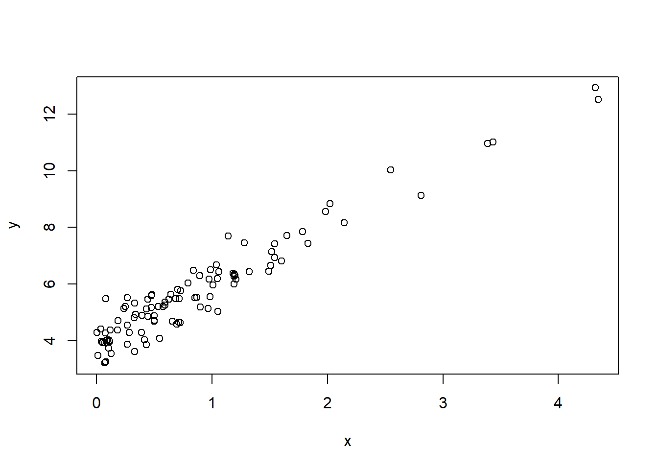

The corresponding R-code to find optimal $k$ and $b$ is the following:

lm(y ~ x, data = df)


Call:
lm(formula = y ~ x, data = df)

Coefficients:
(Intercept)            x  
      3.933        2.071

Here data is the name of the parameter of function lm (stands for “linear model”), and df is the data frame which contains columns x and y. In other words, if columns of df would had names colX and colY, we would write lm(colY ~ colX, data = df).
The (Intercept) corresponds to $b$, and value of x here is $k$. One can access the obtained values:

ans <- coef(lm(y ~ x, data = df))
ans

(Intercept)           x 
   3.932877    2.070541

and then ans[1] is $b$ and ans[2] is $k$.

5.1

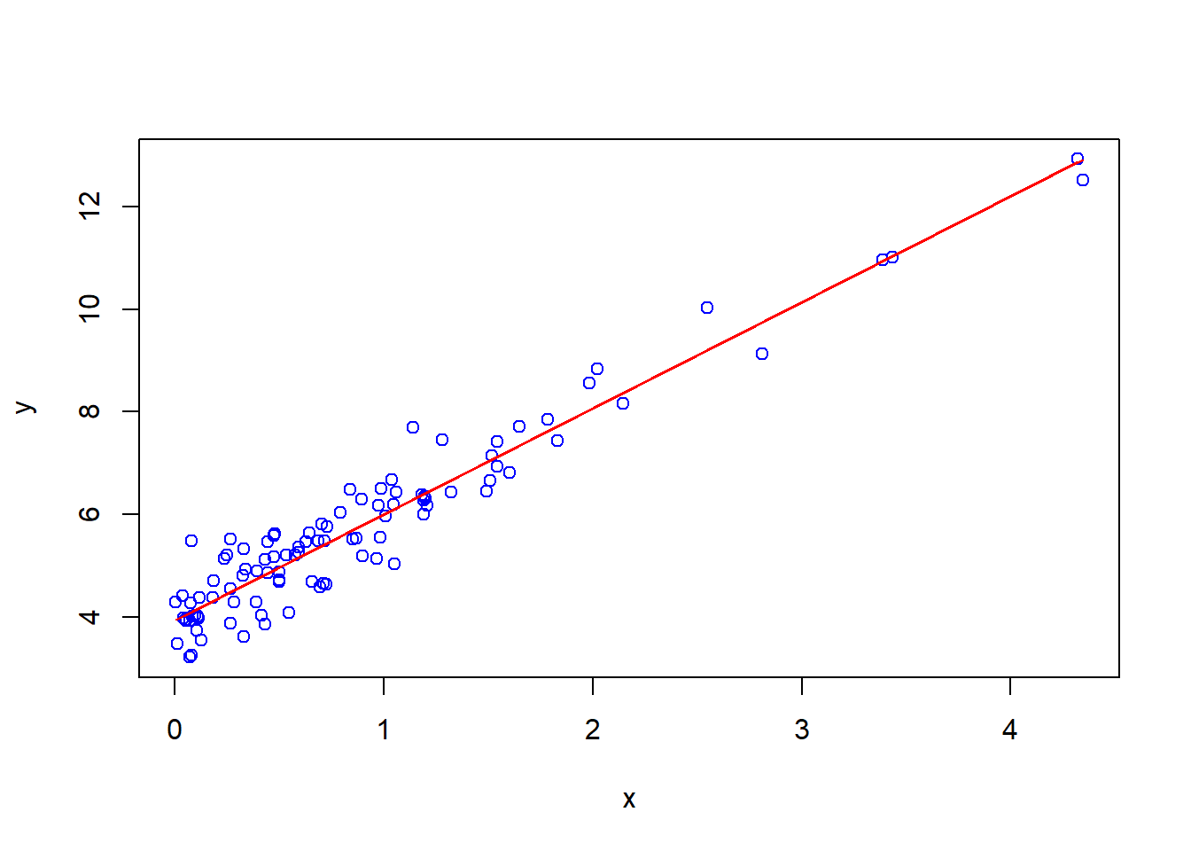
Plot on the same diagram the scatter plot $y$ against $x$ as it is shown above, but in blue color, and plot the line $y=kx+b$ with the found values of $k$ and $b$ (do not copy-paste, use coef function) in red colour. (See Lab 3 for plotting two graphs on one diagram).

Code

x <- df$x
y <- df$y
plot(x, y, col = 'blue')
lines(x, ans[2]*x + ans[1], col = 'red')