Lab 2: Probability Distributions, Plotting, Creating Functions

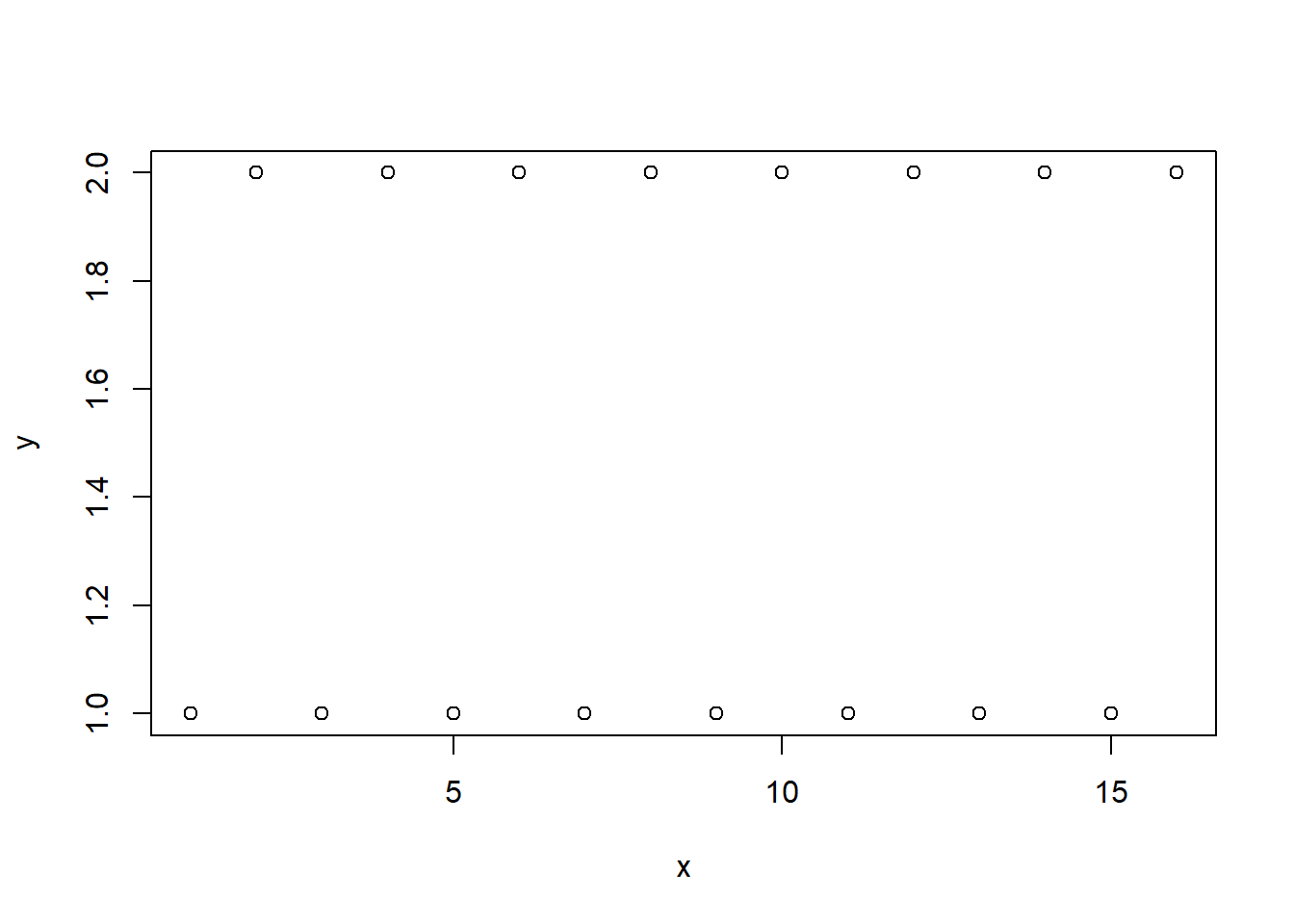
\[ \renewcommand{\P}{\mathbb{P}} \newcommand{\E}{\mathbb{E}} \]

1 Plotting

• To plot values of a vector \(y\) against vector \(x\), we can use plot function, e.g.

x <- 1:16
y <- rep(1:2,8)
plot(x,y)

• To have a graph made by lines, use the following modification

plot(x, y, type='l')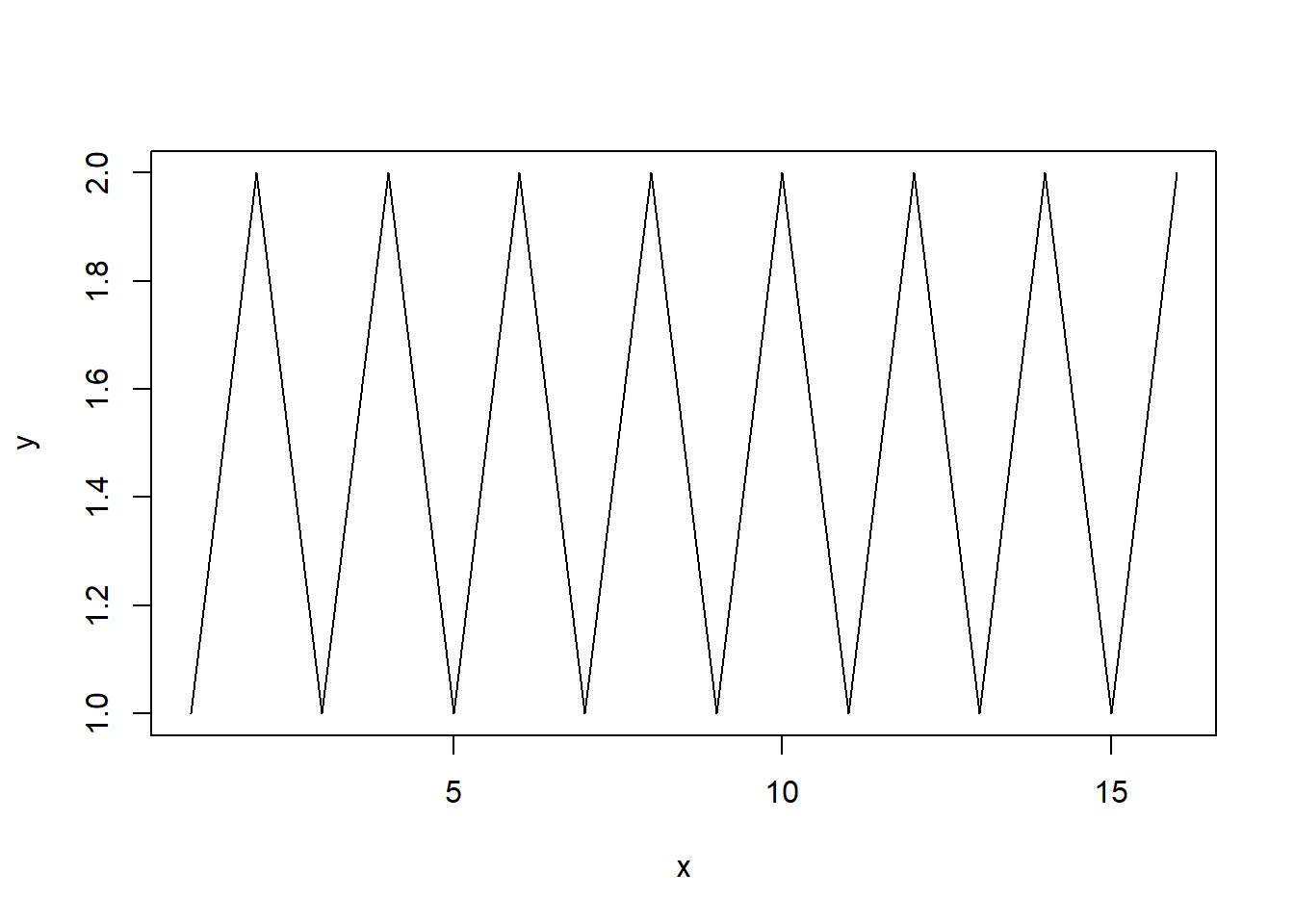

1.1

Plot graph of \(y=x^2\) on \(x\in[-10,10]\). (Hint: divide \([-10,10]\) on many small pieces using seq function discussed in Lab 1, and assign the output of this function to vector x, create vector y of squares of x and, hence, connect values of \(y\) at ends of these pieces by straight lines; if the pieces are small, it would like a smooth curve).

Try by yourself, if it does not work, unfold the code below.

# Recall that R applies any function to a vector component-wise (entry-wise), 
# i.e. if there is a vector `x` and a function `f`, 
# then `f(x)` will be the vector whose first component 
# is the value of `f` on the first compnent of `x` and so on.
x <- seq(-10, 10, 0.1)
y <- x**2
plot(x,y, type='l')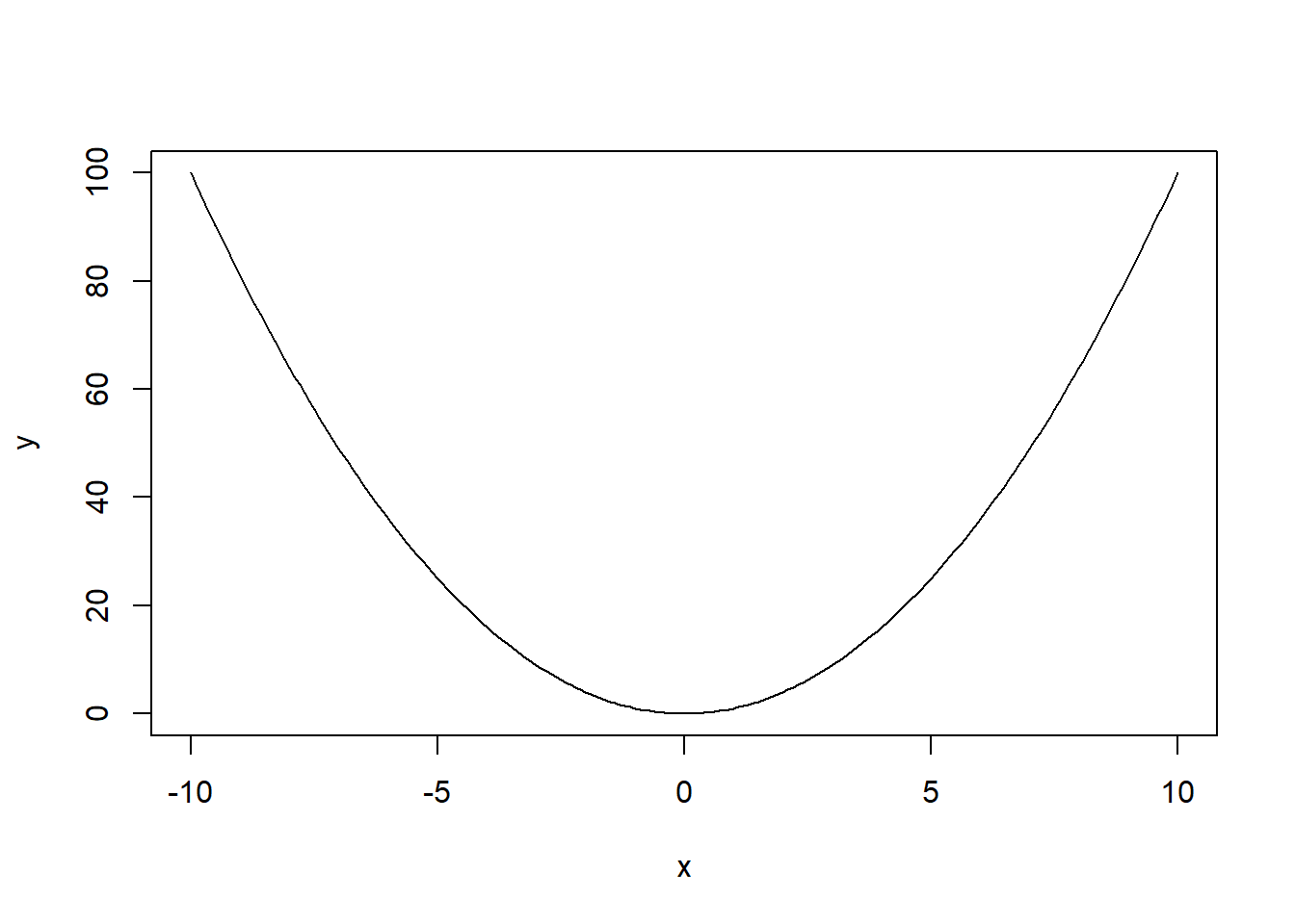

1.2

Let \(X\sim Exp(0.3)\). Plot the graph of the survival function \(S_X(x)\) for \(x\in [0,10]\) using pexp function (also discussed in Lab 1).

The expected output:

x <- seq(0, 10, 0.1)
y <- pexp(x, 0.3, lower.tail = F)
plot(x,y, type='l')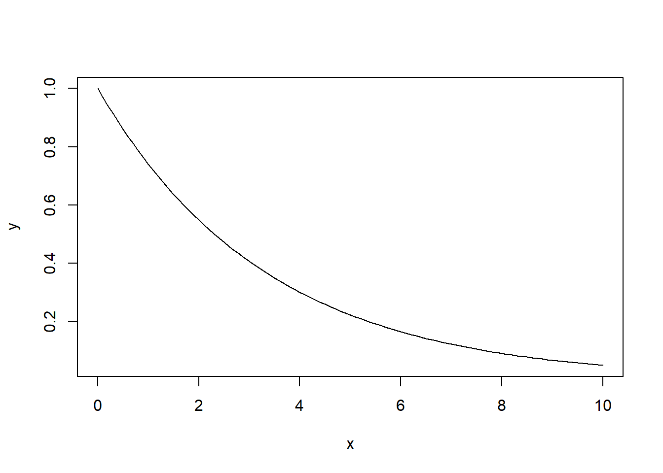

2 Normal and log-normal distributions

• Recall that if \(Z\sim \mathrm{LogN}(\mu,\sigma^2)\), then \(X:=\ln Z \sim \mathrm{N}(\mu,\sigma^2)\).

• In both cases, we have two parameters \(\mu\) and \(\sigma\). Therefore, all functions are “constrcuted” similarly to Gamma distribution from Lab 1, where there were also two parameters.

• For the normal distribution, there are dnorm,pnorm,qnorm,rnorm (PDF, CDF, quntiles, generating of random variables, respectively). The arsuments for \(\mu\) and \(\sigma\) are called mean and sd, respectively.

• Analogously, for the lognormal distribution, the functions are dlnorm,plnorm,qlnorm,rlnorm, and the arguments \(\mu\) and \(\sigma\) are called meanlog and sdlog, respectively.

• In the task below, you will learn about some other arguments of the plot function in R. Each R funciton may have many arguments, and when some of them are missed, the default values are taken. For example, dnorm(5,sd=3) would calculate the value at \(x=5\) of the density of normal distribution with mean \(\mu=0\) and standard deviation \(\sigma=5\). The part mean=0 may be omitted inside the function, because it’s the default value.

2.1

Let \(Y\sim\ln\mathrm{N}(0.01,0.2^2)\). Plot the graph of the density \(f_Y(x)\) for \(x\in[0,3]\). Use xlab and ylab arguments of the plot function to set-up the names “x value” and “Density” for the horizontal and vertical axes. (We didn’t use them before, so their defaults values, which are empty lines, like xlab='', were used by R in the past). Use main argument of the plot function to set-up the title “Normal distribution density” for the whole plot.

Check the output (to make the graph smother, use smaller step in seq function while defining the x values).

x <- seq(0, 3, 0.01)
y <- dlnorm(x, meanlog = 0.01, sdlog = 0.2)
plot(x,y, type="l", xlab="x value", ylab="Density", main="Log-normal distribution density")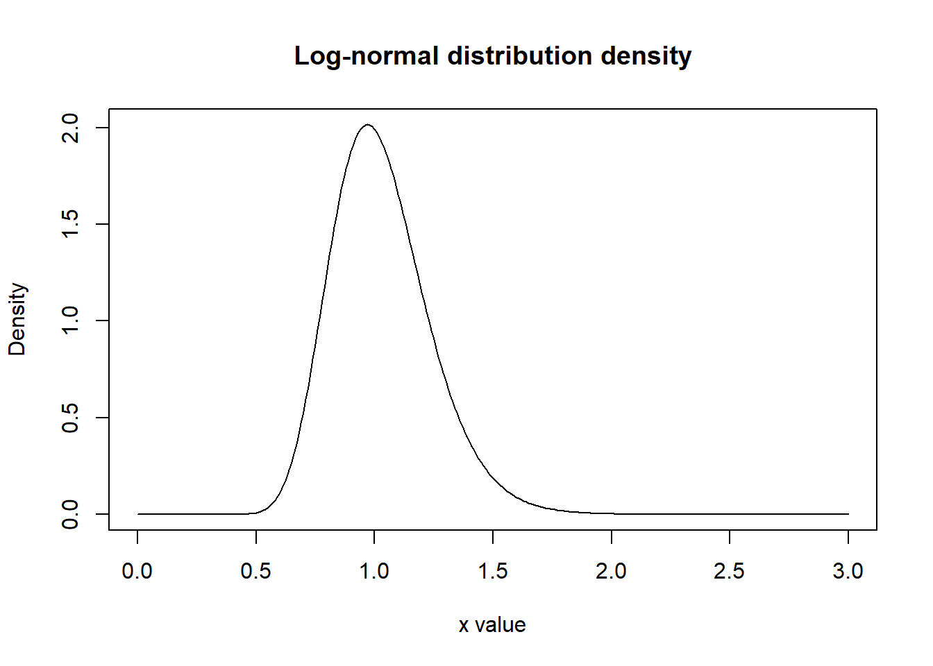

2.2

The hazard function of a random variable \(X\) is defined as follows: \[ h_X(x) := \frac{f_X(x)}{1-F_X(x)}. \] Let \(X\sim \mathrm{N}(4, 0.4)\). Calculate \(h_X(2)\).

Check the output:

sigma = sqrt(0.4) # square root of sigma^2 = 0.4
dnorm(2, 4, sigma)/pnorm(2, 4, sigma, lower.tail = F)

[1] 0.004253513

3 Weibull distribution

• A continuous random variable \(X\) has the Weibull distribution with scale \(\alpha\) and shape \(\beta\), in notations (see Lecture Notes) \(X\sim W(\alpha,\beta)\), if its cumulative distribution function is \[ F(x) = \P(X\leq x) = 1- e^{-\alpha x^\beta}, \qquad x\geq0 \tag{1}\] and its density is, hence, \[ f(x) = \alpha\beta x^{\beta-1} e^{-\alpha x^\beta}. \]

• Also, see Lecture Notes, \[ \E(X)= \Gamma\Bigl(1+\frac{1}{\beta}\Bigr)\alpha^{-\frac{1}{\beta}}. \tag{2}\]

• Then, in particular, the hazard function discussed above can be calculated here explicitly: \[ h(x)=\frac{f_X(x)}{1-F_X(x)}= \alpha \beta x^{\beta-1}. \]

• The corresponding functions built in R use another parametrisation: \[ F(x) = 1- e^{-(x/\sigma)^\beta}, \tag{3}\] i.e. the shape \(\beta\) is the same in both cases, but instead of the parameter \(\alpha\), the parameter \(\sigma\) is in use.

• The scales \(\alpha\) and \(\sigma\) are obviously related: \[ \alpha = \sigma^{-\beta}, \qquad \sigma=\alpha^{-\frac{1}{\beta}}. \tag{4}\]

• Often in the literature \(\alpha\) is called “rate” rather than “scale”.

• The names of built-in functions with the parametrisation as in Equation 3 are dweibull for PDF, pweibull for CDF, qweibull for quantiles, hweibull for the hazard function, and rweibull for generating random values.

• You are advised to specify the name of the argument explicitly, e.g. rweibull(5,shape=0.25,scale=3) would generate \(5\) Weibull random variables with \(\beta = 0.25\) and \(\sigma=3\).

• However, if it is given that e.g. \(X\sim W(0.76,0.25)\) then (at least in our module) we will understand that \(\alpha=0.76\), \(\beta=0.25\) in the notations of Equation 1. Then we can calculate in R the value of \(\sigma\) using a formula from Equation 4, and use the above mentioned functions.

3.1

Set seed 131 (see Task 3.3 of Lab 1). Generate \(10^6\) random variables distributed with \(W(0.76,0.25)\) (i.e. calculate \(\sigma\) from Equation 4 and use the needed function described above); and assign this to a vector. Calculate the sample mean of these values (and assign it to a variable). Calculate the expected value \(\mathbb{E}(X)\) of \(X\sim W(0.76,0.25)\) using Equation 2 and assign it to another variable: note that, for the Gamma-function \(\Gamma(x)\) in Equation 2, you can use R-code gamma(x) (notice the small first letter; e.g. gamma(5) will return 24). Finally, find the absolute value of the difference between the found sample mean and the expected value.

Check your answer:

alpha = 0.76
beta = 0.25
sigma = alpha**(-1/beta)
set.seed(131)
x <- rweibull(10**6, shape=beta, scale=sigma)
m <- mean(x)
e <- gamma(1+1/beta) * alpha**(-1/beta)
abs(m-e)

[1] 0.005210536

• Instead of recalculating the parameters every time we need to use parametrisation Equation 1 instead of the built-in parametrisation Equation 3, we may want to use another functions designed to deal with the parametrisation Equation 1. One can either define needed functions by ourselves or use the functions defined in external libraries (packages).

4 How to define a function

• We start with defining a new function. For example, consider the function which returns, for two variables, the difference of their squares. Let’s call this function sq_diff.

sq_diff <- function(x,y) {
    x**2 - y**2    
}

Then we can use anywhere below, e.g.

sq_diff(4,5)

[1] -9

• Note that a more formal way to define this function would be

sq_diff <- function(x,y) {
    ans <- x**2 - y**2    
    return(ans)
}

The function may contain any number of the code lines.

• In particular, the code inside a function may call another function. For example, the build-in R function sin takes arguments in radians:

sin(pi/6)

[1] 0.5

Let’s define another function which arguments in degrees, recall that \(180^\circ\) is \(\pi\) radians, i.e. \(x^\circ\) is \(\dfrac{x}{180}\pi\) radians. Then we can write

sindeg <- function(x){
    sin(pi*x/180)
}

and then we can use it:

sindeg(30)

[1] 0.5

4.1

Define the function rweibull65 which would have three arguments n, shape, scale, where shape corresponds to \(\beta\) and scale to \(\alpha\) in Equation 1, and which would return n Weibull random values distributed with \(W(\alpha,\beta)\) with shape\(=\beta\) and scale\(=\alpha\); so that this function rweibull65 would call rweibull inside its body; see also the remark below.

rweibull65 <- function(n, shape, scale){
    another_scale <- scale**(-1/shape)
    rweibull(n, shape = shape, scale = another_scale)
}

Run the following code to check your function:

set.seed(12)
rweibull65(2, 1.2, 2.3)

[1] 1.1318101 0.1312781

Remark. R distinguishes the name of the argument and the argument itself. For example, in the defined above function sindeg the argument is called x. So we can specify the argument (though it’s not needed here since it’s the only argument):

sindeg(x = 30)

[1] 0.5

Now, imagine we have a variable in our program which is also called x. Then we can write inside the function x = x:

x <- 30
sindeg(x = x)

[1] 0.5

R will understand that, in x = x the left x is the name of the argument of function sindeg, whereas the right x is the variable defined earlier.

5 How to use an external package

• It should not be surprising that some useful functions (which are absent in the basic R installation) were already created by other people. Such additional function are combined in packages. Each package should be first installed in R Studio and then loaded in R programme (in R-file).

• Note that each package should be installed only once, but it should be loaded in any R-file where it is used.

• We can install package flexsurv which contains functions dweibullPH, pweibullPH, qweibullPH, rweibullPH, hweibullPH which use parametrisation Equation 3. (This package also contains many other useful functions, of course.) To install this package, use menu Tools in R Studio, and select the first item Install Packages... Then you type the package name flexsurv and press Install.

• After this, we write in the code (only once in each Lab file!) library(flexsurv) and then we can use e.g. dweibullPH. For example,

alpha = 0.76
beta = 0.25
sigma = alpha**(-1/beta)
dweibull(1, shape=beta, scale=sigma)

[1] 0.08885662

coincides with

library(flexsurv)
dweibullPH(1, shape=beta, scale=alpha)

[1] 0.08885662

5.1

Let \(X\sim W(1.2, 3.1)\). Using functions pweibullPH and qweibullPH, find \(b\) such that \(\P(1\leq X\leq b)=0.25\).

Check your answer:

# F(b)-F(1)=0.25
# F(b)=F(1)+0.25
fb <- pweibullPH(1, shape=3.1, scale = 1.2)+0.25
b <- qweibullPH(fb, shape=3.1, scale = 1.2)
b

[1] 1.339862

6 Pareto distribution

• Recall that \(X\sim Pa(\alpha,\lambda)\) if \[ F_X(x)=1-\biggl(\frac{\lambda}{\lambda+x}\biggr)^\alpha, \qquad x\geq0. \] and then \[ f_X(x)=\frac{\alpha\lambda^\alpha}{(\lambda+x)^{\alpha+1}} \] and, for \(\alpha>1\), \[ \mathbb{E}(X)=\frac{\lambda}{\alpha-1} \]

• A modification of the Pareto distribution is the Burr distribution with additional parameter \(\gamma>0\) \[ F_{Burr}(x)=F_{Pareto}(x^\gamma)=1-\biggl(\frac{\lambda}{\lambda+x^\gamma}\biggr)^\alpha. \]

6.1

Define function pburr which would have \(4\) arguments: x, alpha, lambda, gamma which would return the value of \(F_{Burr}(x)\) for the given values of the parameters.

pburr <- function(x, alpha, lambda, gamma){
    1 - (lambda/(lambda+x**gamma))**alpha
}

Check your code by calculating \(F_{Burr}(0.5)\) for \(\alpha=1\), \(\lambda=2\), \(\gamma=3\):

pburr(0.5, alpha = 1, lambda = 2, gamma = 3)

[1] 0.05882353

• We discussed previously how to plot the graph of a function. Often we need to plot several graphs on the same diagram, e.g. in different colours. The argument col of function plot is responsible for colours:

x <- seq(-2*pi,2*pi, 0.05)
y <- sin(x)
plot(x, y, col = 'red', type='l')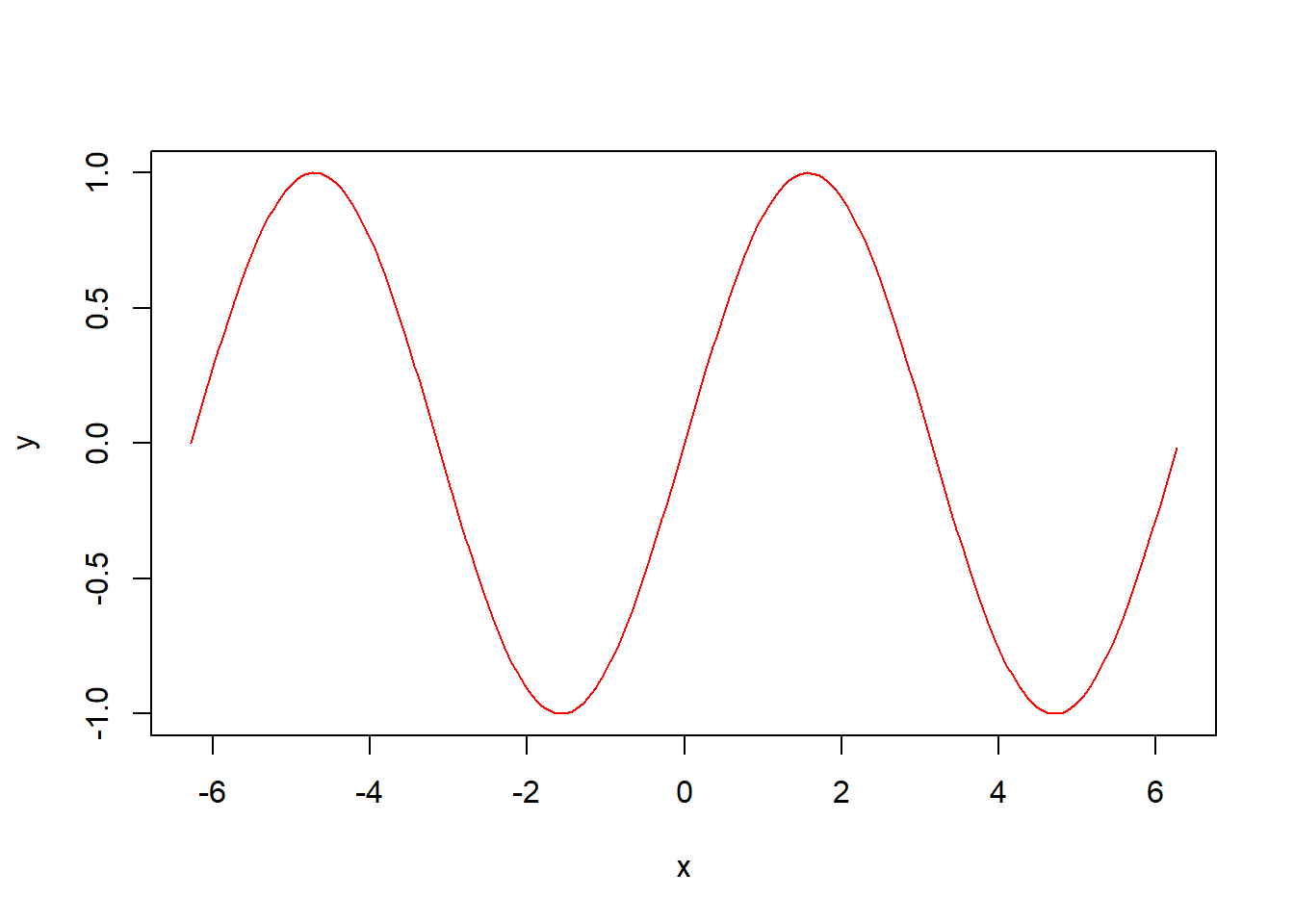

however, to plot another graph we would need to replace the second plot by lines (without type='l'). The last lines add the legend to the graph:

x <- seq(-2*pi,2*pi, 0.05)
y <- sin(x)
z <- cos(x)
plot(x, y, col = 'red', type='l')
lines(x, z, col = 'blue')

legend(x = "topright",          # Position
       legend = c("sin(x)", "cos(x)"),  # Legend texts
       lty = c(1, 1),           # Line types: 1 stands for solid
       col = c('red', 'blue'),  # Line colours
       lwd = 2,                 # Line width
       bg = 'light blue')      # Background color of the legend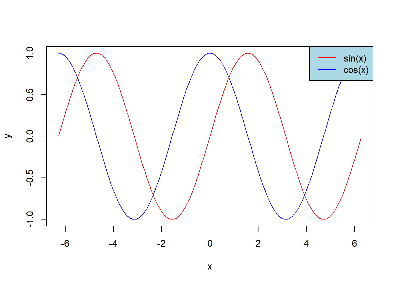  

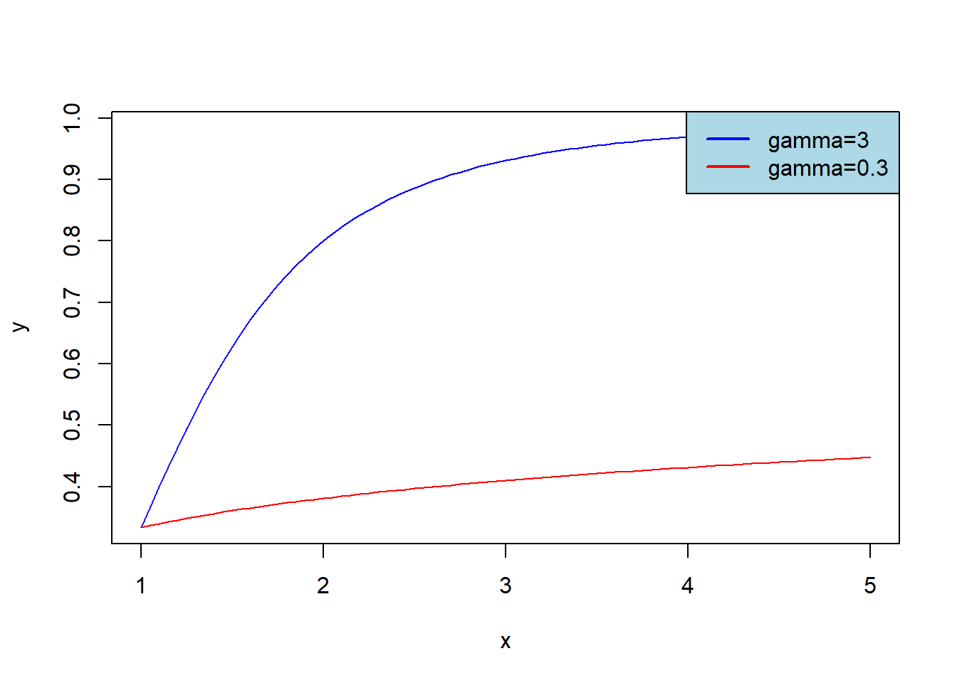
6.2

Plot graphs of \(F_{Burr}(x)\) for \(\alpha=1\), \(\lambda=2\) and \(\gamma=3\) (blue graph) or \(\gamma=0.3\) (red graph); let \(x\in[1,5]\). Add legend to get the result:

x <- seq(1,5, 0.05)
y <- pburr(x, alpha = 1, lambda = 2, gamma = 3)
z <- pburr(x, alpha = 1, lambda = 2, gamma = 0.3)
plot(x, y, col = 'blue', type='l')
lines(x, z, col = 'red')

legend(x = "topright", 
       legend = c("gamma=3", "gamma=0.3"),
       lty = c(1, 1),       
       col = c('blue', 'red'),
       lwd = 2,            
       bg = 'light blue')