5 Continuous Probability Distributions

\[ \renewcommand{\P}{\mathbb{P}} \renewcommand{\E}{\mathbb{E}} \newcommand{\R}{\mathbb{R}} \newcommand{\var}{\mathrm{Var}} \newcommand{\cov}{\mathrm{cov}} \newcommand{\corr}{\mathrm{corr}} \newcommand{\dx}{\,\mathrm{d}x} \newcommand{\dy}{\,\mathrm{d}y} \newcommand{\eps}{\varepsilon} \]

5.1 Continuous Random Variables and their Characteristics

We recall that, see Definition 3.1, a random variable \(X\) is a function \(X:\Omega\to\mathbb{R}\).

Reminder

If \(X\) can take any values from an interval on the real line, then \(X\) is called a continuous random variable.

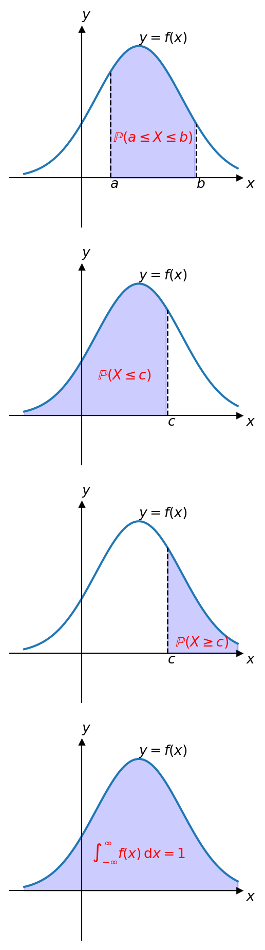
We recall also, see Definition 3.3, that a probability distribution of a random variable \(X:\Omega\to\mathbb{R}\) is a mapping which assigns to each interval \(E\subset\mathbb{R}\) the value of \(\P\bigl(X\in E\bigr)\).

Memorize

The cumulative distribution function (CDF) of a continuous random variable \(X:\Omega\to\mathbb{R}\) is the continuous function \(F_X:\mathbb{R}\to[0,1]\) defined by \[ F_X(x) =\P(X\leq x). \] As a result, \[ \P(a\leq X\leq b) = F_X(b)-F_X(a). \]

Remark. As you can see, the same formula holds for a discrete random variables, however, for continuous r.v. it does not provide an expression to calculate the probability. For this, we need the probaility denisty funciton defined below.

Figure 5.1: Visual representation of probabilities for a continuous random variable

Memorize

The probability density function (PDF) of a continuous random variable \(X:\Omega\to\mathbb{R}\) is the function \(f_X:\mathbb{R}\to[0,\infty)\), such that, for any \(a,b\in\mathbb{R}\), \[ \P(a\leq X\leq b) = \int_a^b f_X(x)\dx. \]

Properties:

\(f_X(x)\geq0\)
\(\displaystyle \int\limits_{-\infty}^\infty f_X(x)\dx =1\)
\(\displaystyle F_X(x)=\int_{-\infty}^x f_X(y)\dy\)
\(\displaystyle f_X(x) = \frac{d}{dx}F_X(x)=F_X'(x)\)

Remember

For conitnuous random variables, \[ \P(X=a)=0, \qquad a\in\mathbb{R}. \] Therefore, \[ \begin{aligned} \P(a\leq X\leq b)&= \P(a\leq X< b)=\P(a< X\leq b)\\ &= \P(a< X< b) = \int_a^b f_X(x)\dx. \end{aligned} \]

Also, the following formulas may be useful: \[ \begin{aligned} \P(X\leq c) &=\P(X< c) = F_X(c)=\int_{-\infty}^c f_X(x)\dx,\\[3mm] \P(X\geq c) & = \P(X> c) = 1- F_X(c)= \int_c^{\infty} f_X(x)\dx. \end{aligned} \]

Recall that the expected value (mean) \(\E(X)\) of a random variable \(X\) is the average value it takes.

Memorize

If \(X:\Omega\to\mathbb{R}\) is a continuous random variable, then \[ \E(X):=\int_{-\infty}^\infty x \cdot f_X(x)\dx \] (provided that the integral takes the finite value).

Remember

More generally, if \(g: \mathbb{R}\to\mathbb{R}\), then \[ \E\bigl( g(X)\bigr) = \int_{-\infty}^\infty g(x) f_X(x) \dx. \] In particular, \[ \E(X^2)= \int_{-\infty}^\infty x^2 f_X(x) \dx. \]

Recall that the variance \(\var(X)\) of a random variable \(X\) is a measure of the spread of its values, and it is defined through the formulas \[ \var(X) = \E\Bigl((X - \E(X))^2\Bigr)=\E\bigl(X^2\bigr) - \bigl( \E(X)\bigr)^2\geq0. \]

Memorize

If \(X:\Omega\to\mathbb{R}\) is a continuous random variable, then \[ \begin{aligned} \var{X} &= \int_{-\infty}^\infty (x-\E(X))^2 f(x)\dx\\& =\int_{-\infty}^\infty x^2\cdot f_X(x)\dx -\biggl( \int_{-\infty}^\infty x\cdot f_X(x)\dx \biggr)^2. \end{aligned} \]

5.2 Main Examples

5.2.1 Uniform distribution

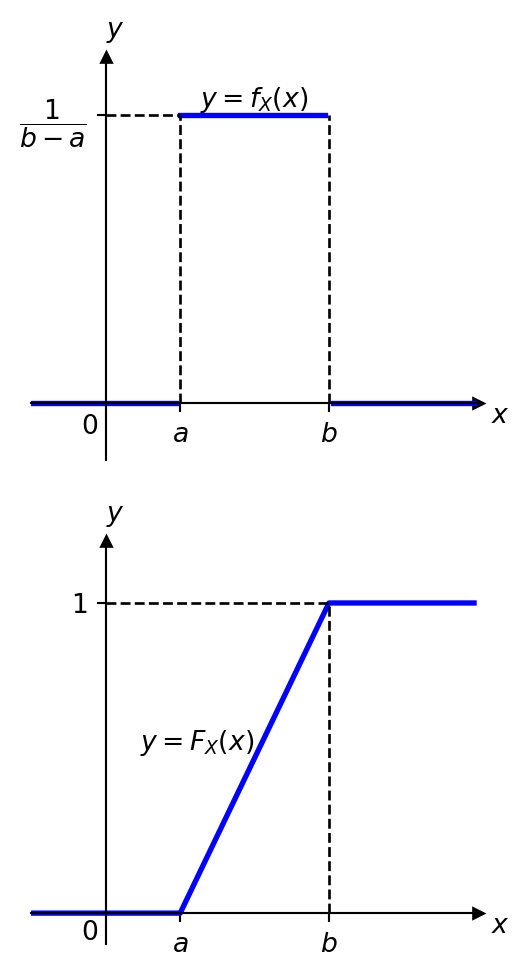
Definition 5.1 The uniform distribution is a continuous probability distribution where all outcomes within a specified interval are equally likely.

Figure 5.2: Graphs of PDF and CDF of \(X\sim U(a,b)\).

Memorize

The PDF of the uniform distribution on an interval \([a,b]\) is given by \[ f(x) = \begin{cases} \dfrac{1}{b-a}, & \text{if } a \leq x \leq b \\[3mm] 0, & \text{otherwise}. \end{cases} \]

The CDF of the uniform distribution on an interval \([a,b]\) is given by \[ F(x) = \begin{cases} 0, & \text{if } x<a\\[3mm] \dfrac{x-a}{b-a}, & \text{if } a \leq x \leq b \\[3mm] 1, & \text{if } x>b. \end{cases} \]

Notation for a random variable with such distribution: \[ X\sim U(a,b). \]

The mean and variance of \(X\) are given by: \[ \begin{aligned} \E(X) & = \dfrac{a+b}{2},\\[2mm] \var(X) & = \dfrac{(b-a)^2}{12}. \end{aligned} \]

Example 5.1 Let \(X\sim U(1,5)\).

Find \(\P(2 < X <4)\).
Find \(c\in[1,5]\) such that \(\P(3 < X <c) = \dfrac13\).

Solution: a) Here \[ f_X(x) = \frac{1}{5-1}=\frac{1}{4}, \qquad x\in[1,5]. \] Therefore, \[ \P(2 < X <4) = \int_2^4\frac14\dx =\frac14\cdot(4-2)=\frac12. \]

We have \[ \dfrac13=\P(3 < X <c)=\int_3^c \frac14\dx=\frac14(c-3), \] hence, \[ c-3=\frac43, \qquad c=\frac{13}{3}\in[1,5]. \]

5.2.2 Exponential Distribution

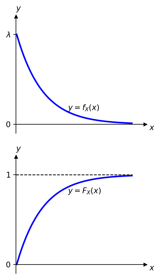
Definition 5.2 Recall that the (discrete) Poisson random variable models the number of independent events occurring in a fixed interval of time.The exponential distribution is a continuous probability distribution that models the time between these independent events. It is commonly used to model waiting times.

Figure 5.3: Graphs of PDF and CDF of \(X\sim \mathrm{Exp}(\lambda)\). Graphs are shown for \(x\geq0\) only. Both functions are equal to \(0\) for \(x<0\).

Memorize

The PDF of the exponential distribution with a parameter \(\lambda>0\) is defined as: \[ f_X(x) = \begin{cases} \lambda e^{-\lambda x}, & \text{if } x \geq 0 \\ 0, & \text{otherwise}. \end{cases} \] The corresponding CDF is \[ F_X(x) = \begin{cases} 1- e^{-\lambda x}, & \text{if } x \geq 0 \\ 0, & \text{otherwise}. \end{cases} \] Notation for a random variable with such distribution: \[ X\sim \mathrm{Exp}(\lambda). \] The mean and variance of \(X\) are given by: \[ \begin{aligned} \E(X) & = \dfrac{1}{\lambda},\\ \var(X) & = \dfrac{1}{\lambda^2}. \end{aligned} \]

Example 5.2 Suppose the time between arrivals at a bus stop follows an exponential distribution with a rate parameter \(\lambda = 0.05\) arrivals per minute.

Calculate the probability that the next bus will arrive within the next \(10\) minutes.
Calculate the probability that you would need to wait at least \(15\) minutes until the next bus.
For how long on average you would need to wait for a bus?

Solution: a) Let \(X\sim \mathrm{Exp}(0.05)\) be the waiting time for the next bus. Then \[ \P(X \leq 10) = F_X(10)= 1 - e^{-0.05 \cdot 10}=1-e^{-0.5}\approx 0.3935. \]

We need to find \[ \P(X\geq15)=1-\P(X<15)=1-F_X(10)=e^{-0.05\cdot 15}=e^{-0.75}\approx 0.4724. \]
Since \[ \E(X)=\frac{1}{0.05}=20, \] you would need to wait, on average, for \(20\) minutes.

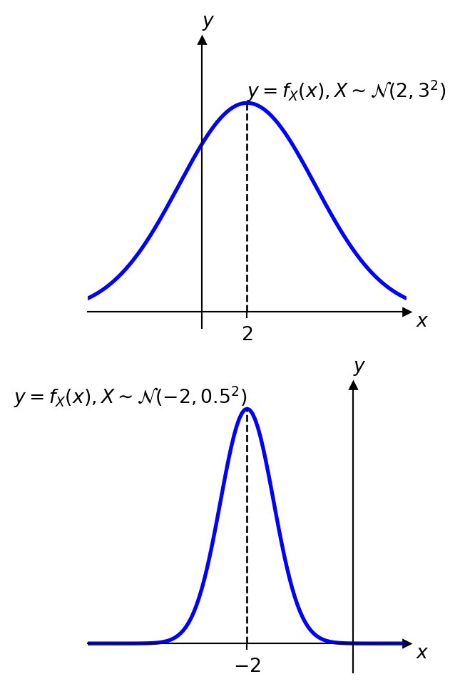
5.2.3 Normal Distribution

Remember

The Normal Distribution is also known as the Gaussian Distribution
The shape of its PDF is symmetric and often called bell-shaped.
The normal distribution is widely used in probability and statistics, especially, because of the central limit theorem which we will discuss later in this course. Its consequence is that the averages of large samples behave simialrly, i.e. “normally”, regardless of the individual behaviour of the elements in these samples.

Figure 5.4: Graphs of PDF of \(X\sim \mathcal{N}(2,3^2)\) and \(X\sim \mathcal{N}(-2,0.5^2)\), respectively.

Memorize

The normal distribution with the mean \(\mu\in\mathbb{R}\) and the standard deviation \(\sigma>0\) is the continuous probability distribution with the PDF given by \[ f_X(x) = \frac{1}{\sqrt{2\pi}\sigma} e^{-\frac{(x-\mu)^2}{2\sigma^2}}. \] Notation for the random variable is \[ X\sim \mathcal{N}(\mu,\sigma^2). \] The names for the parameters \(\mu\) and \(\sigma\) are coming from the relations: \[ \begin{aligned} \E(X)&=\mu,\\ \var(X)&=\sigma^2. \end{aligned} \]

(a) Functions \(\varphi(x)\) and \(\Phi(x)\)

Memorize

The simplest case of a normal distribution is known as the standard normal distribution (or unit normal distribution), and it corresponds to \(\mu=0\), \(\sigma=1\). The PDF of \(X\sim\mathcal{N}(0,1)\) has special notation: \[ \varphi(x):=\frac{1}{\sqrt{2\pi}} e^{-\frac{x^2}{2}}. \] Therefore, if \(X\sim \mathcal{N}(\mu,\sigma^2)\) then \[ f_X(x)= \frac{1}{\sigma}\varphi\biggl( \frac{x-\mu}{\sigma} \biggr). \]

Similarly, for \(X\sim\mathcal{N}(0,1)\), the corresponding CDF is denoted \[ \Phi(x):=\int_{-\infty}^x \varphi(y)\dy=\frac{1}{\sqrt{2\pi}}\int_{-\infty}^x e^{-\frac{y^2}{2}}\dy. \] This function cannot be expressed in terms of elementary functions. To deal with it, one can use computer or statistical tables where its values are given for various values of \(x\) (it’s called that the function \(\Phi\) is tabulated).

It can be shown that if \(X\sim \mathcal{N}(\mu,\sigma^2)\) then the corresponding CDF is \[ F_X(x) = \Phi\biggl( \frac{x-\mu}{\sigma} \biggr). \] There is a standard notation here: \(z=\frac{x-\mu}{\sigma}\), hence, we can rewrite \[ F_X(x)=\Phi(z), \qquad z=\frac{x-\mu}{\sigma}. \]

Note that \[ \Phi(-z) = 1-\Phi(z). \]

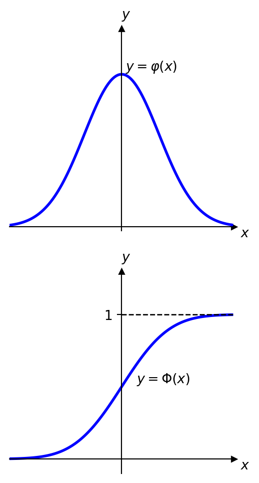
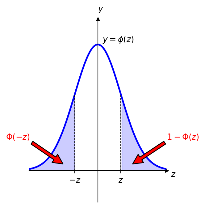
Statistical tables usually provide values of the function \(1-\Phi(z)\) for \(z\geq0\). It gives immediately answer for \(\Phi(-z)=1-\Phi(z)\) and for \(\Phi(z)=1-\bigl(1-\Phi(z)\bigr)\).

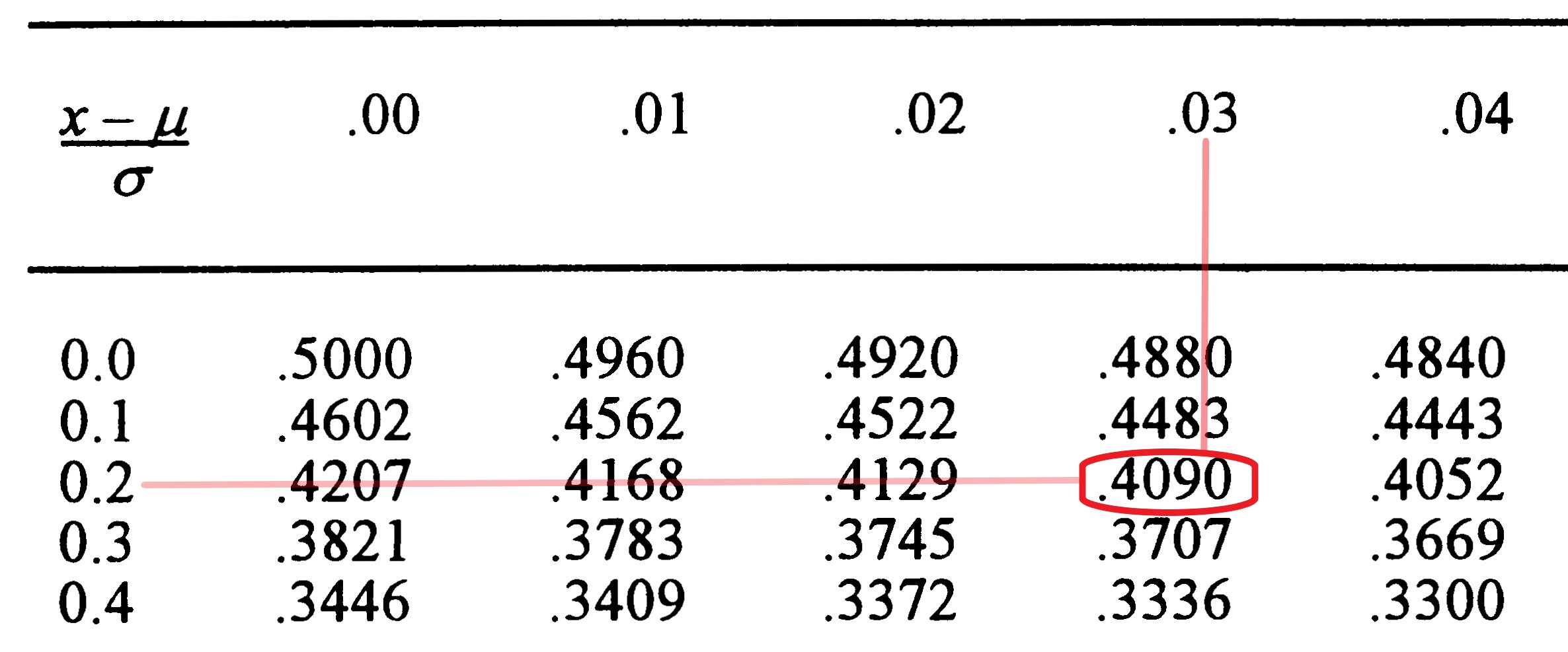
For example, from the statistical table we can find that \[ 1-\Phi(0.23)=0.4090. \] Then \[ \begin{aligned} \Phi(-0.23)&=1-\Phi(0.23)=0.4090,\\ \Phi(0.23)& =1- \bigl( 1-\Phi(0.23)\bigr) = 1-0.4090=0.5910. \end{aligned} \]

Example 5.3 Calculate the probability that a randomly selected individual has a height between \(162\) cm and \(169\) cm, given that the population mean height is \(165\) cm and the standard deviation is \(10\) cm, and that the heights follow the normal distribution.

Solution: Let \(X\) be the random variable representing the height of an individual. It is given then that \(X\sim\mathcal{N}(\mu,\sigma^2)\), where \(\mu=165\), \(\sigma=10\). We need to find \[ \P(162 \leq X \leq 173). \]

First step. We rewrite the required probabiligy in terms of the random variable \[ Z=\frac{X-\mu}{\sigma}, \qquad Z\sim\mathrm{N}(0,1). \] Namely, we have \[ \begin{aligned} \P(162 \leq X \leq 169)&=\P(162 -165\leq X-165 \leq 169-165)\\& =\P(-3\leq X-165 \leq 4)\\& =\P\biggl(-\frac{3}{10}\leq \frac{X-165}{10} \leq \frac{4}{10}\biggr)\\& =\P(-0.3\leq Z \leq 0.4)\\ &=\Phi(0.4)- \Phi(-0.3). \end{aligned} \] From the statistical table (see above), we have that \[ 1-\Phi(0.4)=0.3446, \qquad 1-\Phi(0.3)=0.3821. \] Therefore, \[ \Phi(0.4)=1-0.3446=0.6554, \qquad \Phi(-0.3)=1-\Phi(0.3)=0.3821, \] and hence, \[ \P(162 \leq X \leq 169)= 0.6554-0.3821=0.2733. \]

Surely, we can also use Python:

from scipy.stats import norm
norm.cdf(0.4) - norm.cdf(-0.3)

0.2733331637992768