1 Basic Concepts in Statistics

\[ \renewcommand{\P}{\mathbb{P}} \renewcommand{\E}{\mathbb{E}} \newcommand{\R}{\mathbb{R}} \newcommand{\var}{\mathrm{Var}} \newcommand{\cov}{\mathrm{cov}} \newcommand{\corr}{\mathrm{corr}} \newcommand{\dx}{\,\mathrm{d}x} \newcommand{\dy}{\,\mathrm{d}y} \newcommand{\eps}{\varepsilon} \]

This section will follow closely Chapter 3 of Essential Math for Data Science by T.Nield (see the Reading List on Canvas).

In simple terms, statistics is the collection, analysis and interpretation of data. Data can be qualitative (e.g. hair colour, make of car, etc.) or quantitative (numerical). Data can also be discrete or continuous, where discrete data is distinct, e.g. hair colour and continuous data takes a range of values, e.g. height.

Probability often plays a large role in statistics, as we use data to estimate how likely an event is to happen.

Statistics is the heart of many data-driven innovations. Machine learning in itself is a statistical tool, searching for possible hypotheses to correlate relationships between different variables in data.

We can easily get caught up in what the data says that we forget to ask where the data comes from. These concerns become all the more important as big data, data mining, and machine learning all accelerate the automation of statistical algorithms. Therefore, it is important to have a solid foundation in statistics and hypothesis testing so you do not treat these automations as black boxes.

Definition 1.1

Descriptive statistics involves using tools, for example calculating the mean, median, mode, and using charts, to describe data.

Note that we will recap/cover these concepts shortly.

Definition 1.2

Statistical inference tries to uncover attributes about a larger population, often based on a sample.

Descriptive statistics is the most commonly understood part of statistics and we use it to summarise data. Inferential statistics tries to uncover attributes about a larger population, often based on a sample. It is often misunderstood and less intuitive than descriptive statistics. Often we are interested in studying a group that is too large to observe, for example the average height of adults in the UK, and we have to resort to using only a few members of that group to infer conclusions about them. As you can guess, this is not easy to get right. After all, we are trying to represent a population with a sample that may not be representative.

We next consider populations, samples and bias.

Definition 1.3

A population is the collection of objects or people under discussion, which can be both finite and infinite.

Examples of populations could be “all Swansea University students”, “all adults in the UK”, or “all Golden Retrievers in Scotland”.

If we are going to infer attributes about a population based on a sample, it’s important the sample be as random as possible so we do not skew our conclusions, i.e. we want to avoid bias.

Definition 1.4

A sample is any subset of a population.

In practice it is not often possible/practical to gain information about a whole population therefore we often use a sample of the population instead. We work with samples because we want to make inferences about the population, but clearly there is a risk in coming to a false conclusion by making an inference about the whole population using a sample. Therefore there is a need for statistics tests to ensure that similar results would be obtained if a study were to be repeated and that the results are not just due to sampling variability.

Remark 1.5

It is important to note that populations can be theoretical and not physically tangible. In these cases our population acts more like a sample from something abstract. For example, let us say that we are interested in flights that depart between 2p.m. and 3p.m. at an airport, but we lack enough flights at that time to reliably predict how often these flights are late. Therefore, we may treat this population as a sample instead from an underlying population of all theoretical flights taking off between 2p.m. and 3p.m.

Problems like this are why many researchers resort to simulations to generate data. Simulations can be useful but rarely are accurate, as simulations capture only so many variables and have assumptions built in.

Intuitively, we know that bias is when something is not evaluated in an objective way, however in statistics we have certain types of bias, see below.

Definition 1.6

A. Confirmation bias is gathering only data that supports your belief, which can even be done unknowingly. An example of this is following only social media accounts you politically agree with, reinforcing your beliefs rather than challenging them.

B. Self-selection bias is when certain types of subjects are more likely to include themselves in the experiment. For example, this could be walking onto a flight and polling the customers if they like the airline over other airlines, and using that to rank customer satisfaction among all airlines.

C. Survival bias captures only living and survived subjects, while the deceased ones are never accounted for. For example, many management consulting companies and book publishers like to identify traits of successful companies/individuals and use them as predictors for future successes. These works are pure survival bias, since these works do not account for companies/individuals that failed in obscurity, and these “success” qualities may be commonplace with failed ones as well.

We now look at some descriptive statistics in more detail, beginning with measures of location.

Definition 1.7

The sample mean, denoted by $\bar{x}$, of a sample of observations $x_1, x_2, \ldots, x_n$ is given by \[ \bar{x}=\frac{1}{n} \sum_{i=1}^n x_i=\frac{x_1+x_2+\cdots+x_n}{n}. \]

Analogously, the population mean, denoted by $\mu$, of a population of observations $x_1, \ldots, x_N$ is given by \[ \mu=\frac{1}{N} \sum_{i=1}^N x_i=\frac{x_1+x_2+\cdots+x_N}{N}. \]

Example 1.8 Eight people from the general UK population were polled on the number of pets they own. The results are shown below: \[ 1, 3, 2, 5, 7, 0, 2, 3. \] These are the $x_1, \ldots, x_8$ terms as in the previous definition of the sample mean.Therefore, the sample mean is then given by: \[ \bar{x}=\frac{1+3+2+5+7+0+2+3}{8}=\frac{23}{8}=2.875. \]

Example 1.9 We now modify the situation of the previous example to where the population is now students studying a certain Mathematics module at Swansea University. The values for the whole population are as follows: \[ 2,1,3,4,2,6,4,0,1,1,3,3,4,1,1,5,5,2,1,3. \]

The population mean is then given by: \[ \begin{aligned} \mu&=\frac{2+1+3+4+2+6+4+0+1+1+3+3+4+1+1+5+5+2+1+3}{20}\\ &=\frac{52}{20}=2.6. \end{aligned} \]

Definition 1.10

We define the weighted mean by \[ \frac{x_1\cdot w_1+x_2\cdot w_2+\cdots+x_n\cdot w_n}{w_1+w_2+\cdots+w_n}, \] where $x_1,\ldots,x_n$ denote the observations and $w_1,\ldots,w_n$ are the corresponding weights.

Example 1.11 Let us consider a module with three coursework components worth 20% each and a final exam that is worth 40%. A student scores $90, 80, 63$ and 87 respectively in these components. The weights are therefore 0.2, 0.2, 0.2 and 0.4 respectively and the weighted average is given by, \[ \frac{0.2\cdot90+0.2\cdot80+0.2\cdot63+0.4\cdot87}{0.2+0.2+0.2+0.4}=81.4. \]

Definition 1.12

The median is the middle value of ranked data if $n$ is odd and it is the mean of the two middle values if $n$ is even, i.e. \[ \frac{\frac12n^{\text{th}}+(\frac12n+1)^{\text{th}}}{2}. \]

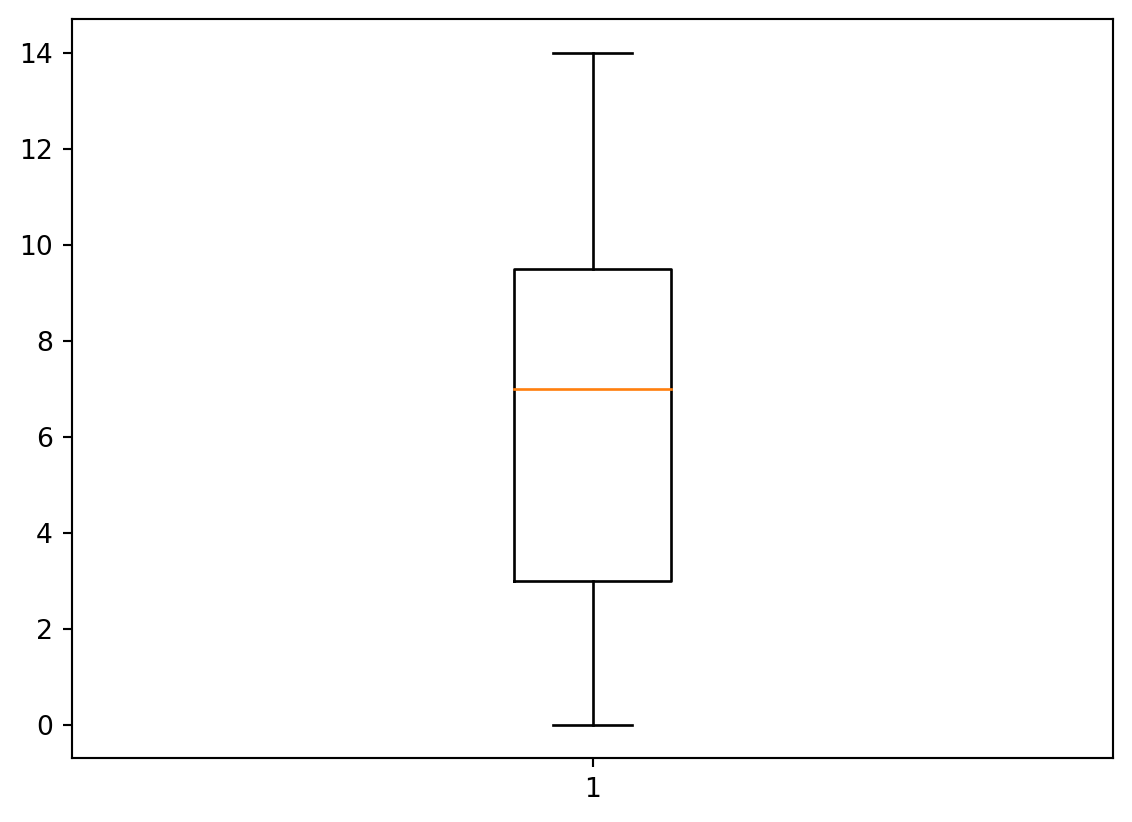
Example 1.13 Calculate the median of the values: 5,0,1,9,7,10,14. Firstly we rank these values to obtain: \[ 0,1,5,7,9,10,14. \] Since $n$ is odd (i.e. 7) we take the middle value of 7 to be the median. If we now add one value of 20 to this example, then the modified ranked data is given by: \[ 0,1,5,7,9,10,14,20. \] Now we have an even number of values (i.e. 8) and hence the median is given by $\tfrac{7+9}{2}=8$.

Remark 1.14

There is a concept of quantiles in descriptive statistics. The concept of quantiles is essentially the same as a median, just cutting the data in other places besides the middle. The median is actually the 50% quantile, or the value where 50% of ordered values are behind it. Then there are the 25%, 50%, and 75% quantiles, which are known as quartiles because they cut data in 25% increments.

Definition 1.15

The mode is the most frequently occurring set of values. It primarily becomes useful when your data is repetitive and you want to find which values occur the most frequently.

Example 1.16 Find the mode of the values $20,21,19,20,22,19,20$. The most common value is 20, hence 20 is the mode of this dataset.

The mode is not necessarily unique, see the example below for an illustration.

Example 1.17 If we return to Example 1.8, we find that the mode for the number of pets is 2 and 3.

We now consider measures of variation of data. This gives us a sense of how “spread out” the data is. It is important to note that there are some calculation differences for the sample versus the population.

Definition 1.18

A. For a population of data values $x_1,\ldots,x_N$, the (population) variance is given by, \[ \sigma^2=\frac{\sum_{i=1}^N(x_i-\mu)^2}{N}, \] where $\mu$ is the mean of the population. Furthermore, the (population) standard deviation is the square root of the variance, i.e. \[ \sigma=\sqrt{\frac{\sum_{i=1}^N(x_i-\mu)^2}{N}.} \]

B. For a sample of data values $x_1,\ldots,x_n$, the sample variance is given by, \[ s^2=\frac{\sum_{i=1}^n(x_i-\bar{x})^2}{n-1}, \] where $\bar{x}$ is the sample mean. Similarly, the sample standard deviation is the square root of the sample variance, i.e. \[ s=\sqrt{\frac{\sum_{i=1}^n(x_i-\bar{x})^2}{n-1}.} \]

Remark 1.19

Note that for the sample variance (and hence the sample standard deviation) we divide by $n-1$ rather than the total number of items. We do this to decrease any bias in a sample and not underestimate the variance of the population based on our sample. By counting values short of one item in our divisor, we increase the variance and therefore capture greater uncertainty in our sample.

Example 1.20 In this example we are interested in studying the number of pets owned by members of staff in a certain shop (note that this is our population, not a sample). The data are as follows: \[ 0,14,5,9,7,10,1. \] The mean of this sample is 6.571, hence the variance is given by

\[ \begin{aligned} \sigma^2&=\frac{\sum_{i=1}^N(x_i-\mu)^2}{N}\\ &=\text{\scriptsize{$\dfrac{(0-6.571)^2+(14-6.571)^2+(5-6.571)^2+(9-6.571)^2+(7-6.571)^2+(10-6.571)^2+(1-6.571)^2}{7}$}}\\ &=21.29. \end{aligned} \]

Therefore the standard deviation is given by $\sigma=\sqrt{21.38}=4.62$. (All to 2dp.)

Example 1.21 We now modify the previous example to the situation where the data provided are a sample of a larger population. We now calculate the sample variance and standard deviation: \[ \begin{aligned} s^2&=\frac{\sum_{i=1}^n(x_i-\bar{x})^2}{n-1}\\ &=\text{\scriptsize{$\dfrac{(0-6.571)^2+(14-6.571)^2+(5-6.571)^2+(9-6.571)^2+(7-6.571)^2+(10-6.571)^2+(1-6.571)^2}{6}$}}\\ &=24.95. \end{aligned} \]

Therefore the sample standard deviation is given by $\sigma=\sqrt{24.95}=4.99$. (All to 2dp.)

Notice that the sample variance and standard deviation have increased compared to the population case. This is correct as a sample could be biased and imperfect representing the population. Therefore, we increase the variance (and thus the standard deviation) to increase our estimate of how spread out the values are. A larger variance/standard deviation shows less confidence with a larger range.

Definition 1.22

Measures of characteristics of a sample are called statistics. (Not to be confused with the subject area of statistics described above.) The corresponding characteristics in the population are called parameters.

We work with samples because we want to make inferences about the population, but clearly there is a risk in coming to a false conclusion by making an inference about the whole population using a sample. Therefore there is a need for statistics tests to ensure that similar results would be obtained if a study were to be repeated and that the results are not just due to sampling variability.

The final topic of this chapter discusses some basic data visualisation techniques - in particular, we will consider histograms, box plots and scatter plots.

Definition 1.23

A histogram is a graphical display of continuous data using bars. A bar chart provides a graphical display of categorical data.

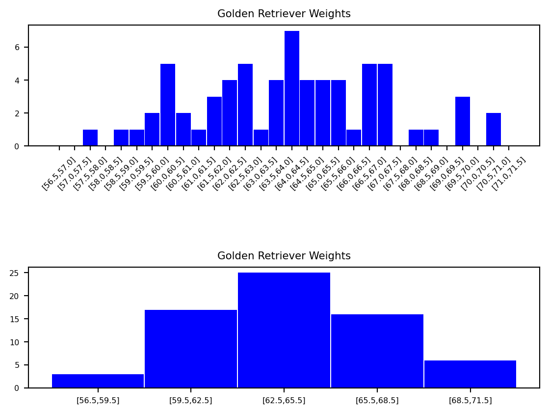
Note that there are no gaps between the bars of histograms and the bars can be of varying widths, i.e. they may have different sized intervals or `bins’. Histograms can be used to help determine the distribution of the data.

Example 1.24 In this example we consider the weight of Golden Retrievers. See below for examples of histograms for this data.

This histogram does not reveal any meaningful shape to our data. The reason is because our bins are too small.

As you can see, if we get the bin sizes just right (in this case, each has a range of three pounds), we start to get a meaningful bell shape to our data.

Definition 1.25

A box plot or a box-and-whisker plot is a graphical technique to display data using quartiles. The box itself indicates the interquartile range, i.e. the 25% quartile to the 75% quartile. The median is indicated by a line within the box. The end of the lower (or left) whisker indicates the minimum and the top of the upper (or right) whisker denotes the maximum. Outliers are usually indicated by points.

Box plots are useful to visualise the distribution of data, in particular to check for symmetry.

Example 1.26 Let us use the data in Example 1.13 to produce the following box plot.

Definition 1.27

We obtain bivariate data when we measure two variables on each member of the population or sample.

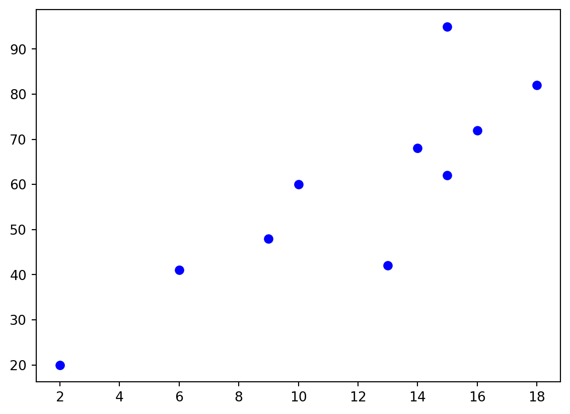
Scatter plots can be used to plot such data, these plots can also help to visualise a relationship between the variables. One variable is plotted on the horizontal axis and the other on the vertical axis.

Example 1.28 Let us consider the data below which records exam marks for students and the corresponding time (in hours) the students spent revising for the exam.

This can be represented by the following scatter plot: