2 Basic Concepts and Rules of Probability

\[ \renewcommand{\P}{\mathbb{P}} \renewcommand{\E}{\mathbb{E}} \newcommand{\R}{\mathbb{R}} \newcommand{\var}{\mathrm{Var}} \newcommand{\cov}{\mathrm{cov}} \newcommand{\corr}{\mathrm{corr}} \newcommand{\dx}{\,\mathrm{d}x} \newcommand{\dy}{\,\mathrm{d}y} \newcommand{\eps}{\varepsilon} \]

2.1 Introduction to Probability Theory

Probability Theory is a branch of mathematics that deals with uncertainty and randomness. It provides a framework for quantifying and analyzing uncertainty in stochastic experiments.

Probability theory plays a crucial role in data science, where we often deal with uncertain data and make predictions based on probabilities.

An experiment or trial is any procedure that can be infinitely repeated and has a well-defined set of possible outcomes.

An outcome (denoted by \(\omega\)) is a particular result of an experiment.

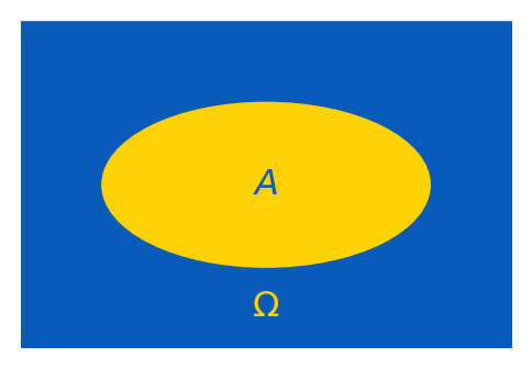
A sample space (denoted by \(\Omega\)) is the set of all possible outcomes of an experiment (i.e. \(\omega\in\Omega\)).

An event is a subset of the sample space (e.g. \(A\subset \Omega\)), representing a specific outcome or a collection of outcomes.

Probability (denoted by \(\P\)) is a measure of the likelihood of an event occurring. It assigns a number between \(0\) and \(1\) to an event, where \(0\) indicates extreme unlikelihood, and \(1\) indicates certainty that the event will occur. In particular, \[0\leq \P(A)\leq \P(\Omega) = 1.\]

Example 2.1 When we throw a coin ones, the possible outcomes are \(H, T\) (stand for ‘head’ and ‘tail’).

Therefore, \(\Omega=\{H, T\}\).

There are \(4\) events one can consider: \(\{H\}, \{T\}, \{H,T\}, \emptyset\).

Example 2.2 Consider rolling a fair six-sided dice.

The possible outcomes then are \(1,2,3,4,5,6\).

Therefore, \(\Omega=\{1,2,3,4,5,6\}\).

Consider the event \(A\) of getting an even number: \(A = \{2, 4, 6\}\).

Consider the event \(B\) of getting a prime number: \(B = \{2, 3, 5\}\).

Then \(\P(A)=\P(B)=\frac12\) (think why).

Remember

The event \(\emptyset\) (‘empty set’) describes an impossible event (e.g. we throw a coin or a dice with no outcome). Then \[ \P(\emptyset) = 0. \]

Remark. In the experiment from Example 2.2, the following \(2^6=64\) events can be considered \[ \begin{gathered} \emptyset, \{1\}, \{2\}, \ldots, \{6\},\\ \{1,2\}, \{1,3\}, \ldots, \{5,6\},\\ \{1,2,3\}, \ldots, \{4,5,6\},\\ \ldots\\ \{1,2,\ldots,6\}. \end{gathered} \]

Remember

If the sample space \(\Omega\) contains \(n\) elements (outcomes), then the set of all events (that is the set of all subsets of \(\Omega\)) is denoted by \(2^\Omega\), and it contains \(2^n\) events.

Memorize

We start our course with the discrete case, when \(\Omega\) is a finite set. To calculate the probability \(\P(A)\) of an event \(A\subset\Omega\), we use the following formula: \[ \P(A)=\dfrac{\textrm{number of outcomes that make } A}{\textrm{number of all outcomes}}=\dfrac{\sharp(A)}{\sharp(\Omega)} \]

Figure 2.1: Visual representation of \(\P(A)=\dfrac{\color{myYellow}\mathbf{oval}}{\color{myBlue}\mathbf{rectangle}}\)

Example 2.3 Consider rolling twice a fair six-sided dice. Then outcomes are \(\omega=(a,b)\) where \(a,b\in \{1, 2, 3, 4, 5, 6\}\), i.e. \[ \Omega = \bigl\{ (a,b) \mid a,b\in \{1, 2, 3, 4, 5, 6\} \bigr\}. \] Then \(\sharp(\Omega)=6\cdot 6=36\). Let \(A\) be the event of having the sum of the numbers in two rollings bigger than \(10\). Then \[ A=\bigl\{ (5,6), (6,5), (6,6) \bigr\}. \] Therefore, \[ \P(A)=\frac{3}{36}=\frac1{12}. \]

Example 2.4 Consider drawing a card from a standard deck of \(52\) playing cards. The sample space \(\Omega\) is the set of all \(52\) pairs of the form \(vS\), where \(v\in\{A, 2, 3, 4, \ldots, 10, J, Q, K\}\) is the value of a card (here \(J\) represents a Jack, \(Q\) represents a Queen, \(K\) represents a King, and \(A\) represents an Ace), and \(S\in\{\clubsuit,{\color{red}\diamondsuit}, \spadesuit, {\color{red}\heartsuit}\}\) is the card suit (e.g. \(2{\color{red}\diamondsuit},\ldots, A{\color{red}\diamondsuit}\) are all diamonds). Let \(B\) be the event of drawing a red face card. Then \[ B=\{J{\color{red}\diamondsuit}, Q{\color{red}\diamondsuit}, K{\color{red}\diamondsuit}, J{\color{red}\heartsuit}, Q{\color{red}\heartsuit}, K{\color{red}\heartsuit}\}, \] and hence, \[ \P(B)=\frac{6}{52}=\frac{3}{26}. \]

2.2 Rules of Probability

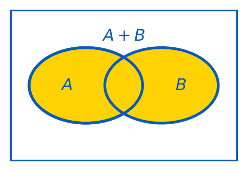
Definition 2.5 The sum of events \(A\) and \(B\) is the event \(A+B\) (also denoted \(A\cup B\) or \(A\vee B\)) which occurs iff either \(A\) occurs or \(B\) occurs or they both occur.

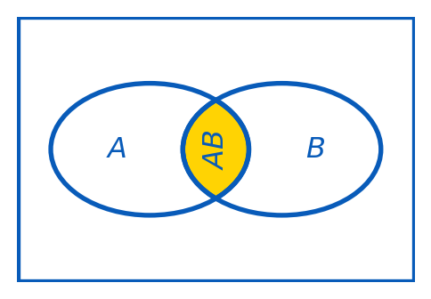
Figure 2.2: Visual representation of \(A+ B\)

Definition 2.6 The product of events \(A\) and \(B\) is the event \(AB\) (also denoted \(A\cap B\) or \(A\wedge B\)) which occurs iff both \(A\) and \(B\) occur.

Figure 2.3: Visual representation of \(AB\)

Remember

\(A+B\) occurs under more outcomes than either of \(A\) or \(B\) alone: \[ \P(A+B) \geq \P(A), \quad \P(A+B) \geq \P(B). \]
\(AB\) occurs under less outcomes than each of \(A\) or \(B\) alone: \[ \P(AB) \leq \P(A), \quad \P(AB) \leq \P(B). \]

Memorize

The addition rule states that \[ \P(A + B) = \P(A) + \P(B) - \P(A B). \] It can be easily interpretted using the visual representations of \(\P(A + B)\) and \(\P(AB)\).

Example 2.7 There is a standard deck of \(52\) playing cards. Find the probability of drawing either a red card or a face card (king, queen, or jack) from the deck in a single draw.

Solution: Let \(A\) be the event of drawing a red card, and \(B\) be the event of drawing a face card. Overall, there are \(26\) red cards, \(12\) face cards, and \(6\) red face cards. Therefore, \[ \P(A+B)=\frac{26}{52}+\frac{12}{52}-\frac{6}{52}=\frac{32}{52}=\frac{8}{13}. \]

Remember

Events \(A\) and \(B\) are called mutually exclusive events if only one of them may happen, i.e. if \(AB=\emptyset\). In this case \(\P(AB)=0\), and the addition rule takes the form \[ \P(A+B)=\P(A)+\P(B). \]

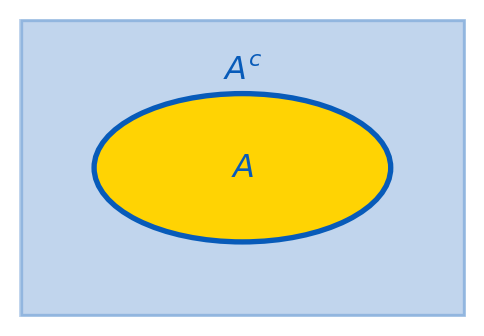
Definition 2.8 The complement to an event \(A\) is the event \(A^c\) which occurs iff \(A\) does not occur. Since \(\P(\Omega)=1\), one has \[ \P(A^c)=1-\P(A). \]

Figure 2.4: Visual representation of \(A^c\)

Example 2.9 A fair six-sided dice is rolling three times. Find the probability that the total score (the sum of three trials) will be at least \(4\) (event \(A\)).

Solution: The sample space \(\Omega\) consists of all triples \((a,b,c)\) with \(a,b,c\in\{1,2,\ldots,6\}\). Thus, \(\sharp(\Omega)=6^3=216\). The total score is \(4\) or more in all cases but the case \((1,1,1)\). Therefore, the answer is: \[ \P(A) = 1-\P(A^c)=1-\frac{1}{216}=\frac{215}{216}. \]

Definition 2.10 Conditional probability \(\P(A\mid B)\) is the probability of an event \(A\) occurring given that event \(B\) has already occurred, so we assume that \(\color{red}\P(B)\neq0\). The formula is \[ \P(A\mid B) = \frac{\P(AB)}{\P(B)}. \]

Memorize

The multiplication rule follows immediately from the formula for the conditional probability: \[ \P(AB) = \P(B)\, \P(A\mid B) = \P(A)\, \P(B\mid A). \]

Remember

The multiplication rule can be generalised for the product of several events, e.g. \[ \P(ABC) = \P(A) \, \P(B\mid A)\,\P(C\mid AB). \]

Example 2.11 In a bag of \(20\) marbles, \(8\) are red, and \(12\) are green. Three marbles are drawn from the bag without replacement. What is the probability that they all are of the same color?

Solution: we need to find the probability that either \(A=(r,r,r)\) or \(B=(g,g,g)\) holds. Note that \(A\) and \(B\) are mutually exclusive events. By the multiplication rule, \[ \P(A) = \frac{8}{20}\cdot\frac{7}{19}\cdot\frac{6}{18}, \] and \[ \P(B) = \frac{12}{20}\cdot\frac{11}{19}\cdot\frac{10}{18}. \]

Therefore, by the addition rule (for mutually exclusive events), \[ \P(A+B)=\P(A)+\P(B)=\frac{8\cdot 7\cdot 6}{20\cdot 19\cdot 18}+\frac{12\cdot 11\cdot 10}{20\cdot 19\cdot 18}=\frac{1656}{6840}=\frac{23}{95}. \]

Definition 2.12 An event \(A\) is said to be independent on an event \(B\) if the occurrence of \(B\) does not affect the probability of occurrence of \(A\). In other words, \(A\) is independent on \(B\) iff \[ \P(A\mid B) = \P(A). \]

Example 2.13 A fair coin is tossing twice. Let \(A\): a head appeared in the first tossing, and \(B\): a tail appeared in the second tossing. Then \(A\) and \(B\) are independent. \(A=\{HH,HT\}\), \(B=\{HT,TT\}\), and hence, \(AB=\{HT\}\). Then \(\P(AB)=\frac14=\frac12\cdot\frac12=\P(A)\P(B)\).

Remember

If \(A\) is independent on \(B\) then \(B\) is independent on \(A\), and \[ \P(AB)=\P(A)\,\P(B). \]

Remark. If three (or more) events are pairwise independent: \(A\) and \(B\) are independent, the same for \(B\) and \(C\), and for \(A\) and \(C\), it still may be that they are not independent in total, and then, in general, \(\P(ABC)\neq\P(A)\P(B)\P(C)\) (see the multiplication rule).

Figure 2.5: Note that \(A=AB_1+\ldots +AB_n\)

Memorize

Let \(B_1,\ldots,B_n\) be pairwise exclusive events (i.e. \(B_iB_j=\emptyset\) for all \(i\neq j\)) such that \(B_1+B_2+\ldots+B_n=\Omega\) with \(\P(B_i)\neq0\) (it is said then that \(B_1,\ldots,B_n\) form a partition of \(\Omega\)). Then the law of total probability holds: \[ \P(A)=\P(A\mid B_1)\,\P(B_1)+\ldots+\P(A\mid B_n)\,\P(B_n). \]

Remember

There is also a modification of the law of total probability for conditional probabilioties. If \(B_1,\ldots,B_n\) are as above and \(\P(C)\neq0\), then \[ \P(A\mid C) = \P(A\mid B_1 C)\P(B_1\mid C)+ \ldots + \P(A\mid B_n C)\P(B_n\mid C). \]

From Definition 2.10, we have that \[ \P(B) \P(A\mid B) = \P(AB)=\P(BA)=\P(A)\P(B\mid A). \] This implies the following important statement.

Memorize

Let \(\P(A)\neq0\) and \(\P(B)\neq0\). Then Bayes’ rule (a.k.a. Bayes’ formula or Bayes’ theorem) holds: \[ \P(A\mid B) = \frac{\P(A)\P(B\mid A)}{\P(B)}. \] It describe the a posteriori probability of the event \(A\), after an experiment with the known outcome \(B\), using the a priori information about the outcome \(B\).

Remember

If \(A_1,\ldots,A_n\) form a partition of \(\Omega\) (i.e. \(A_1+\ldots+A_n=\Omega\) and \(A_iA_j=\emptyset\) for \(i\neq j\)) with \(\P(A_j)\neq0\), then we can rewrite Bayes’ rule as follows, for \(\P(B)\neq0\): \[ \P(A_i\mid B) = \dfrac{\P(A_i)\P(B\mid A_i)}{\displaystyle\sum_{j=1}^n\P(B\mid A_j)\P(A_j)}. \]

Example 2.14 A patient has taken a test for a rare disease. The prevalence of the disease in the population is known to be very low, only \(0.1\)%. The test correctly identifies the disease in \(95\)% of cases when it’s present. The test incorrectly indicates the presence of the disease in \(3\)%, of cases where it’s not actually present. The patient has just received a positive test result for the disease. What is the probability that he actually has the disease?

Solution: Let \(D\) denote the event of having the desease for a member of the population, then \(\P(D) = 0.001\) (\(0.1\)%). Let \(T\) denote the event of the positive test result. Then we know that \[ \P(T|D) = 0.95, \qquad \P(T|D^c) = 0.03. \] By the very definition, \(D\) and \(D^c\) form a partition of \(\Omega\). Then \[ \P(D|T) = \frac{\P(T|D) \cdot \P(D)}{\P(T|D) \cdot \P(D) + \P(T|D^c) \cdot \P(D^c)} = \frac{0.95 \cdot 0.001}{0.95 \cdot 0.001 + 0.03 \cdot (1 - 0.001)} \approx 0.0306. \] So, given a positive test result for the disease, the probability that the patient actually has the disease is just \(3.06\)%.