Lab 2 - Solutions

1 First calculations of probabilities

1.1

A fair coin is tossed 25 times. Store at the variable a the probability to get 25 heads. A fair six-sided dice is throwing 10 times. Store at the variable b the probability to get 10 equal even scores. Find the ratio a/b.

Solution. The probability of a head is \(0.5\), and all tossings are independend, hence, the probability to get \(n\) heads in a row is

\[ 0.5^n. \]

Next, \(m\) equal even scores in \(m\) throwings of the dice may be in \(3\) cases:

\[ (\underbrace{2,\ldots,2}_{m\ \mathrm{times}}), (\underbrace{4,\ldots,4}_{m\ \mathrm{times}}), (\underbrace{4,\ldots,4}_{m\ \mathrm{times}}) \] These cases are mutually exclusive, hence the probability that either of them happens is the sum of probabilities of each event. Each probability is equal to

\[ \Bigl(\frac16\Bigr)^{m}, \] hence, for b, we need to multiply the latter number (for \(m=10\)) by \(3\).

Code

#
a = 0.5 ** 25
b = 3 * (1/6) ** 10 # Read about the order of operations in Python
a/b

0.6006774902343753

1.2

An experiment consists of selecting a token from a bag and spinning a coin. The bag contains \(345\) red tokens and \(678\) blue tokens. A token is selected at random from the bag, its colour is noted and then the token is returned to the bag.

When a red token is selected, a biased coin with probability \(\dfrac45\) of landing heads is tossed.

When a blue token is selected, a biased coin with probability \(\dfrac25\) of landing heads is spun.

Find the probability c of obtaining tail. Round the answer to 3 decimal digits.

Solution. Let \(R\) and \(B\) be the events of selecting a red (respectively, blue) token. Then

\[ \mathbb{P}(R) = \frac{345}{345+678},\qquad \mathbb{P}(B) = 1-\mathbb{P}(R)= \frac{678}{345+678}. \]

Let \(T\) be the event of obtaining a tail. We will use the total probability law:

\[ \mathbb{P}(T) = \mathbb{P}(T\mid R)\cdot \mathbb{P}(R)+ \mathbb{P}(T \mid B)\cdot \mathbb{P}(B). \]

We know also that \(\mathbb{P}(H\mid R)=\frac45\), hence, \(\mathbb{P}(T\mid R)=1-\frac45=\frac15\). Similarly, \(\mathbb{P}(T\mid B)=1-\frac25=\frac35\).

Code

p_red =  345/(345+678)
p_blue = 1 - p_red
c = p_red * (1 - 4/5) + p_blue * (1 - 2/5)
round(c, 3)

0.465

1.3

In the conditions of the previous task, if the tail was obtained, what is the probability \(d\) of having selected a red token? Round the answer to 3 decimal digits.

Solution. By Bayes’ formula,

\[ \mathbb{P}(R | T) = \frac{\mathbb{P}(R) \cdot \mathbb{P}(T | R)}{\mathbb{P}(T)} \]

Code

d = p_red * (1-4/5) / c
round(d, 3)

0.145

2 Combinatorics

Memorize

Factorial of a natural (i.e. positive integer, or positive whole) number \(n\) is the product of all numbers from \(1\) to \(n\). It’s denoted \(n!\), i.e.

\[ n! = 1\cdot 2\cdot \ldots \cdot n. \]

It is also set that

\[ 0! = 1 \]

We can calculate factorial manually, e.g. using a loop:

n = 10
f = 1
for i in range(2,n+1):
    f *= i          # this is the same as f = f * i
f

We can also use a special function:

import math
math.factorial(10)

There is also another large library, called scipy which contains factorials and many other scientific functions. Note, however, the additional parameter.

from scipy.special import factorial
factorial(10, exact=True)       # Try without 'exact', notice the difference

Memorize

Let \(n\) and \(k\) be natural numbers such that \(k\leq n\). The number of \(k\)-element subsets of an \(n\)-element set is called the binomial coefficient \(\binom{n}{k}\) (it reads as “\(n\) choose \(k\)”) and it can be calculated by the formula

\[ \binom{n}{k}=\frac{n!}{k! \cdot (n-k)!} \]

In Python, we can use the following code, to get the number of \(4\)-element subsets of a \(10\)-element set

from scipy.special import comb
n = 10
k = 4
comb(n, k, exact=True)

2.1

In a school sport club, there are \(20\) children who like rugby more than football, and \(15\) chidlren who like football more than rugby. (Noone likes them equally.) The club wants to form a committee of \(6\) people: \(3\) football funs and \(3\) rugby funs. How many ways does there exist to form the committee? Store the answer in w.

Remark. Note that since the choice of football funs does not depend on the choice of rugby funs, we need just to multiply the number of ways to choose fotball funs and the number of ways to choose rugby funs.

Solution. Therefore,

\[ w = \binom{20}{3}\cdot\binom{15}{3} \]

Code

w = comb(20,3, exact=True) * comb(15,3, exact=True)
w

2.2

Let now the committee (of 6 children) is chosen without any restrictions on the preferences of its members. Find the number of ways to form the committee. Store the answer in r.

Solution. We choose \(6\) children from \(20+15=35\), it can be done in \(\binom{35}{6}\) ways.

Code

# We choose 6 children from 35
r = comb(35,6, exact=True)
r

2.3

Finally, find the probability p that a randomly choosen committee consisting of 6 children has equal numbers of football and rugby funs. Round to \(4\) decimal digits.

Code

p = round(w/r,4)
p

0.3196

2.4

If \(10\) balls are randomly drawn from a bag containing \(17\) blue and \(19\) yellow balls, what is the probability q that \(4\) of the balls are blue and the others are yellow? Round to \(3\) decimal digits.

Note that despite the balls of the same colour are indistinguishable (in contrast to children of the same sport preference in the previous tasks), we may always think that the balls e.g. numbered, to apply the same arguments as before.

Code

q = comb(17, 4) * comb(19, 10-4) / comb(17+19, 10)
q

0.25404208941472567

Remember

Special cases:

\[ \binom{n}{0}=\binom{0}{0}=1 \]

Simple cases:

\[ \binom{n}{1} = n, \qquad \binom{n}{2}=\frac{n(n-1)}{2} \]

Overall,

\[ \binom{n}{k} = \frac{n\cdot(n-1)\cdot(n-2)\cdot\ldots\cdot(n-k+1)}{1\cdot2\cdot3\cdot\ldots\cdot k}, \]

where numerator has \(k\) factors. E.g.

\[ \binom{37}{4}=\frac{37\cdot 36\cdot 35\cdot 34}{1\cdot 2\cdot 3\cdot 4}. \]

3 How to model simple random events

To model various random events in Python, we may use module random:

import random

Lets model tossing a fair coin. Define the list

coin = ['h','t']

Command random.choice(list_name) would return a randomly chosen element from a list list_name assuming that any such an element can be picked with equal probability.

3.1

Choose a random element from the list coin. The output will be one of two letters h or t, e.g.:

Code

random.choice(coin)

't'

Note that if you run the same code again and again you may get each time another output.

Congratulations: you made your first probability model.

3.2

Suppose we tossed the coin n_trials = 10 times. Generate a list called series that would contain outputs of all these trials, e.g.

Code

n_trials = 10
series = [random.choice(coin) for _ in range(n_trials)]
series

['t', 'h', 'h', 't', 'h', 't', 't', 't', 't', 't']

(your output will be probably different).

Advice: it may be more convenient to use list comprehension instead of loops, though it’s up to you. Recall that range(10) command generates 10 numbers from 0 to 9.

Count the number of “heads” in series, using property list_name.count(element_name) to get the number of elements element_name in the list list_name.

Code

series.count('h')

3.3

Load library pyplot of module matplotlib as follows:

import matplotlib.pyplot as plt

Change now n_trials to 1000. We expect to see around 500 heads in a series of trials, though if you run your code, you will probably get another number. Define n_series = 1000 and repeat running the previous code n_series times, i.e. the output should be a list of n_series numbers. Store the output in a variable heads.

Again, you may find more useful to use list comprehension.

Create the scatter plot of numbers of heads in all series using the commands plt.scatter(x, heads) and plt.show(), where x would be all numbers from 0 to n_series.

Your output should be similar to:

Code

#The first line of the code is to see the output in Jupyter notebook
%matplotlib inline
n_trials = 1000
n_series = 1000
heads = [[random.choice(coin) for _ in range(n_trials)].count('h') for _ in range(n_series)]
x = range(n_series)
plt.scatter(x, heads)
plt.show()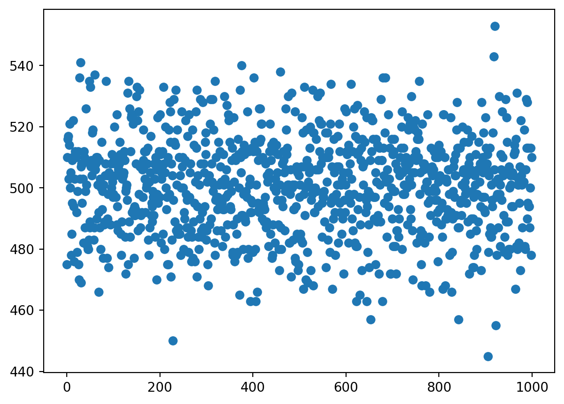

As you can see all results indeed gather around 500. Note that you can find min(heads) and max(heads) to see how large is the spread of numbers, e.g. on the picture above it’s

[min(heads),max(heads)]

[445, 553]

4 When you have free time

Of course, our approach may become very time-consuming when n_series becomes large. There exist special functions for generating big amounts of random values. The following code generates n = 10 random integer numbers from the interval \([0,2)\) (i.e. either \(0\) or \(1\)):

import numpy as np
n = 10
a = np.random.randint(2, size=n)
a

array([1, 0, 0, 0, 1, 0, 0, 0, 1, 0])

We may think then that \(0\) stands for h and \(1\) stands for t (or vice versa). Then the number of tails is the number of \(1\) in a, that is just the sum of all elements from a. Note that despite sum(a) would work, for large values of n, the following code will be faster:

s = a.sum()
s

If now we want to repeat the previous code \(5\) times, getting each time a number s of tails, we may use the following modification of the code:

a_series = np.random.randint(2, size=(5,n))
a_series

array([[1, 1, 1, 0, 0, 0, 0, 0, 0, 0],
       [0, 1, 1, 0, 0, 1, 1, 0, 1, 0],
       [1, 0, 0, 1, 1, 0, 1, 1, 0, 0],
       [0, 0, 0, 1, 1, 1, 0, 0, 0, 0],
       [1, 1, 0, 0, 0, 0, 0, 1, 1, 0]])

and also

s_series = a_series.sum(axis=1)
s_series

array([3, 5, 5, 3, 4])

We can also calculate the average of obtained numbers (their sum divided by their quantity):

s_series.mean()

4.0

4.1

Consider again that we toss the coin \(1000\) times and count the number of tails, but repeat this procedure \(10^5\) times. Calculate the average m of the obtained result.

Code

n = 1000
b = np.random.randint(2, size=(10**5,n))
b.sum(axis=1).mean()

500.00904

As expected, the result is pretty close to \(500\) (your result may differ from this, of course).

4.2

We can also model unfair coins. The command

n=10
np.random.choice([0,1], size=(5,n), p=[0.6, 0.4])

array([[1, 1, 1, 1, 0, 0, 0, 1, 1, 0],
       [0, 0, 1, 1, 1, 0, 0, 0, 0, 0],
       [1, 1, 0, 0, 1, 1, 0, 0, 0, 0],
       [1, 1, 0, 0, 0, 0, 0, 1, 0, 0],
       [0, 1, 0, 1, 0, 0, 0, 0, 0, 0]])

generates \(5\) series of \(10\) outputs each with the probability for head \(0.6\) and the probability for tail \(0.4\). Calculate again the average for \(10^5\) series of \(1000\) trials.

Code

n = 1000
b = np.random.choice([0,1], size=(10**5,n), p=[0.6, 0.4])
b.sum(axis=1).mean()

399.91953

The result is pretty close to \(400 = 0.4*1000\). We discuss the theoretical justification for this on Week 3.